BIT-101
Bill Gates touched my MacBook Pro
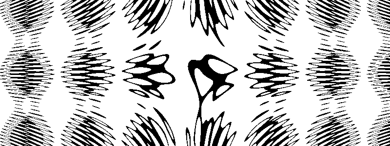
This post is about programming strategies for graphing various equations and functions. I often see some interesting graph and an accompanying equation or functions and I want to recreate it and play with it a bit and see what else I can do with it. The thing is, there are a few different ways these things can be presented. So I’ll go through some of these and we can explore some strategies.
Functions are pretty easy in general. If you think back to your school days, a mathematical function looks something like this: y = f(x), where f(x) = x + 3 for example. Pretty similar to programming functions and you can usually map between the two pretty easily. An important thing to remember about functions is that for any given x, there will always be exactly one y.
So say we had f(x) = sin x. Easy. We create a function in code like so (in somewhat JavaScript-y pseudocode):
function firstFunc(x) {
  return sin(x)
}
Now we can run through a bunch of x values, say from 0 to the width of our canvas, and get y values for each of them and draw segments. Maybe something like:
for (x = 0; x < width; x++) {
  y = firstFunc(x)
  lineTo(x, y)
}
stroke()

Now you just see some blips on the top edge of the canvas. So we need to do a few things to adjust the range of the output graph. Move it down a bit, increase the amplitude and wavelength. You can do this by translating and scaling but that can have resolution side effects, so we’ll do it with math.
for (x = 0; x < width; x++) {
  y = firstFunc(x * 0.1) * 40 + 50
  lineTo(x, y)
}
stroke()
I multiply x by 0.1 to increase the wavelength. Multiply the result of firstFunc by 40 to increase the amplitude, and add 50 to that to move it down to the center of the image.

Notice that for each point on the x-axis, there is exactly one point it matches on the y-axis. So functions are pretty easy. But what if you have something like a circle?
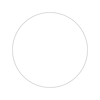
For some x values there is no corresponding y value. And for some there are two y values. So this is not a function and we need to do something else.
Parametric equations take a parameter (or multiple parameters). For two-dimensional graphs, there’s often two functions based on the same parameter. One function returns the x coordinate of a point, and the other returns the y coordinate. In this case, I’m using “function” in the less strict, or programming sense.
It’s common in trigonometric parametric equations to have the parameter be called “theta” and is often defined by the letter t. In these cases, theta is an angle that can range from 0 to 2 PI. The parametric equation(s) for a circle might then look like:
function circle(t) {
  x = cos(t)
  y = sin(t)
  return x, y
}
My theoretical pseudocode language allows returning two values from a function. If your real world language doesn’t, you might have to return some kind of point object.
Now you can draw a circle by passing in a series of t values from 0 to 2 PI
for (t = 0; t <= 2 * PI; t += 0.01) {
  x, y = circle(t)
  lineTo(x * radius, y * radius)
}
stroke()
Since this circle function will just return values from -1 to 1, I multiplied them by a radius value. You could also offset the circle on the canvas as well. You might want to make radius and center point additional parameters to the function.
Note that the amount you increase t by (0.01 in this case) will affect the resolution of the circle. Increase it by too much on each iteration and you’ll get something more like a polygon. Increase it by too little and you’ll get a super smooth circle, but you might be doing way more work than you need. The trick is finding the balance.
For a more interesting parametric equation, we can turn to the rose curve.
The equation for a rose curve is r = a * cos(n * t). This equation takes three parameters:
a is the amplitude - kind of the max radius of the rose.n is the number of nodes in the curve.t as usual is theta.The result of this equation is not an x, y point just yet, but a radius corresponding to a particular theta angle. We can turn that into a function that returns x, y by using cosine and sine on t, multiplying the result by r. It will look like this:
funcion rose(a, n, t) {
  r = a * cos(n * t)
  return cos(t) * r, sin(t) * r
}
And we can use it like so:
for (t = 0; t <= 2 * PI; t += 0.01) {
  x, y = rose(150, 5, t)
  lineTo(200 + x, 200 + y)
}
stroke()
In this case, since the returned point has a useful radius, I just translate it by 200 on both axes to center the shape. Here’s the result:
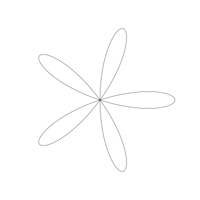
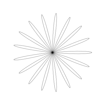
And if I increase n to 17, we get that many nodes:
This gets even more interesting if you make n a rational fraction, like 11/13. In this case however, it will take more cycles to get all the way back to the starting point. 13 * PI does the trick.
for (t = 0; t <= 13 * PI; t += 0.01) {
  x, y = rose(150, 11.0/13.0, t)
  lineTo(200 + x, 200 + y)
}
stroke()
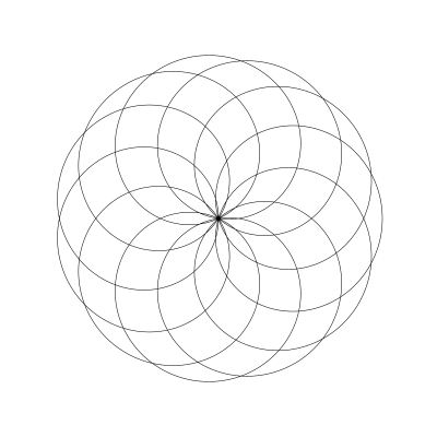
There are a lot of parametric equations that return a radius. Now you know how to handle them.
Often you’ll come across an equation that isn’t in parametric form. For example, the standard form of the circle equation is:
(x - h)^2 + (y -k)^2 = r^2
Or, in code…
pow(x - h, 2) + pow(y - k, 2) == pow(r, 2)
Any set of x, y, h, k values that satisfies that equality is part of the circle. And we can rewrite this by taking the square root of each side, like so:
sqrt(pow(x - h, 2) + pow(y - k, 2)) == r
Now normally, for a circle, we wouldn’t even bother with this form, because we already know the parametric form. But let’s give it a shot as a simple use case for how to deal with things that are represented this way.
One strategy is to look at every point on the canvas and see if it satisfies that equation. So we loop through x from 0 to the canvas width and y from 0 to its height and plug those numbers into the formula. If the conditional is true, we color that pixel. Something like this:
h = 200
k = 200
r = 150
for (x = 0; x < width; x++) {
  for (y = 0.0; y < height; y++) {
    if sqrt(pow(x - h, 2) + pow(y - k, 2)) == r {
      fillRect(x, y, 1, 1)
    }
  }
}
Here, h and k define the center of the circle and r is its radius.
And that gives us…
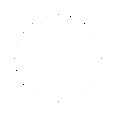
…almost nothing. You can see a few points on the edge of the circle, but not many. The reason for this is that we’re being way to strict. We’re rarely going to find an x, y point that is exactly on the circle. if it’s even 0.00000001 of a pixel off, that’s a false. So we need to build in wiggle room. If it’s close enough to equal that’s ok.
So we say that square root value is the distance from the center of the circle. If that’s exactly equal to the radius, then the difference is 0 and we want to plot that point. To give us that wiggle room, we can say if the difference between the distance and the radius is less than a small amount, that’s close enough. We’ll subtract the two and we’ll take the absolute value to get the actual un-signed distance.
h = 200
k = 200
r = 150
for (x = 0; x < width; x++) {
  for (y = 0.0; y < height; y++) {
    dist = sqrt(pow(x - h, 2) + pow(y - k, 2))
    if abs(dist - r) < 0.5 {
      fillRect(x, y, 1, 1)
    }
  }
}
Here I checked to see if that difference is less than 0.5, which gives us this:
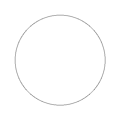
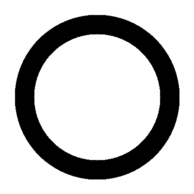
Of course if we increase that value, we can get a circle with a much wider boundary. Here I’m comparing to see if the distance is less than 20.
OK, now I said normally we wouldn’t use this method for something as simple as a circle where we already have a better method. But what if you have an equation like this?
sin(sin(x) + cos(y)) = cos(sin(x * y) + cos(x))
I’m not sure there even is a parametric form of something like this, or how I’d go about finding it. But we can pretty easily plot this the same way we just did for the circle.
There will be a few steps to go through though. First we want to map our x and y canvas pixel values to a much smaller range. -14 to 14 will work well. I’m going to use the map function I described in this post:
I’ll assign the mapped x, y values to xx and yy
for (x = 0; x < width; x++) {
  for (y = 0.0; y < height; y++) {
    xx = map(x, 0, width, -14, 14)
    yy = map(y, 0, height, -14, 14)
  }
}
Now I’ll put those values into both sides of that equation. I’ll do this separately, calling the first one a and the second one b. Then I’ll see if they match to within a certain distance, and if so, plot that point.
for (x = 0; x < width; x++) {
  for (y = 0.0; y < height; y++) {
    xx = map(x, 0, width, -14, 14)
    yy = map(y, 0, height, -14, 14)

    a = sin(sin(xx) + cos(yy))
    b = cos(sin(xx * yy) + cos(xx))

    if abs(a-b) < 0.25 {
      fillRect(x, y, 1, 1)
    }
  }
}
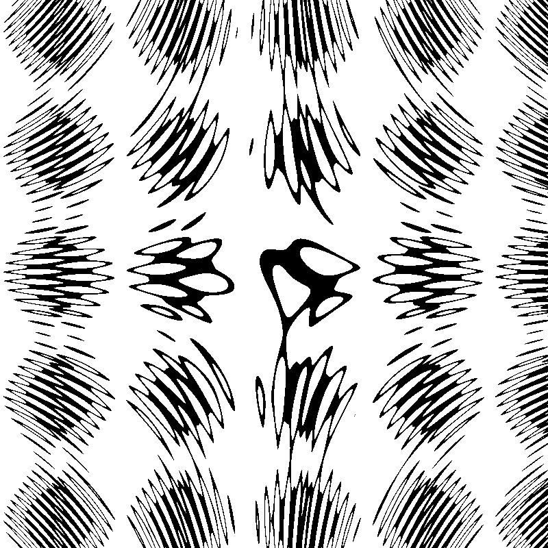
You can try setting different values in the map function to zoom in and out, and different values to compare the distance to. Here I used 0.25. Smaller values will make thinner lines and shapes. Higher values will give a more blobby look.
Then start experimenting with the equation itself. And find other equations to graph. And animate them. And…