Chapter 4 in the Coding Curves Series

Make sure you are familiar with at least the first chapter, to understand how the code samples work.

Lissajous curves have always been one of my favorite techniques. They are useful for many things beyond the obvious loopy shapes they create. In this installment, we’ll cover the basics, and as usual, wander off course here and there to look at other ways they can be used.

The Basics

Lissajous curves are also known as Lissajous figures or Bowditch curves. Both names came from the names of men who looked into and wrote about them in the 1800s.

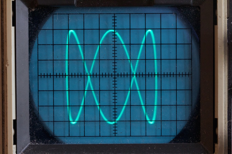
These figures are formed by long looping curves that go back and forth and left and right. In their pure form, they recall the glowing patterns seen on oscilloscopes used for special effects in a vintage scifi movies.

The Formula

In this case, a useful parametric formula was one of the first things I found in researching this subject.

x = A * sin(a * t + d)
y = B * sin(b * t)

Basically what we have here is a sine wave on the x-axis, and another sine wave on the y-axis. So instead of going off infinitely in any direction, it keeps looping back in on itself.

We have a bunch of variables here. Let’s break them down.

A and B wind up being the width and height of the curve on the x- and y-axes. Or technically, half the width and height because the curve will extend that distance in each direction.

The t is a parametric variable that will range form 0 to 2 * PI. Although it can actually go beyond that in either direction, it will effectively just loop back on itself when it does. t is multiplied by a for the x component, and by b for the y component, and the sine is taken of the result on each axis. In addition, the x component has a d or delta variable added to it to move it out of phase.

This formula might look a bit familiar from the previous chapter on circles. If we set A and B equal to each other and call them r, and set a and b both equal to 1, then remove the d and use cosine instead of sine for the x component, then we get:

x = r * cos(t)
y = r * sin(t)

This is the parametric formula for a circle (with its center at 0, 0). Since cosine is the same as sine but 90 degrees out of phase, we could also say:

x = r * sin(t + d)
y = r * sin(t)

… where d equals 90 degrees, or PI / 2 radians.

You can also see the relation to the ellipse formula if you keep A and B separate, where A is what we called the “x radius” and B is the “y radius”:

x = A * sin(t + d)
y = B * sin(t)

So when everything is in sync like this, we get a circle or ellipse, but when we start changing these parameters, we get much more interesting curves.

OK, enough talk, let’s code. We can jump right into making a Lissajous function. I’ll abbreviate a bit.

function liss(cx, cy, A, B, a, b, d) {
  res = 0.01
  for (t = 0; t < 2 * PI; t += res) {
    x = cx + sin(a * t + d) * A
    y = cy + sin(b * t) * B
    lineTo(x, y)
  }
  closePath()
}

Here, the resolution value is not as straightforward as in circles and ellipses. For now, I’m just going to keep the res value very small, even if it means we’re doing to much work for simpler, smaller curves. Since we’re going from 0 to 2 * PI (6.28…), incrementing by 0.01 will give us 628 line segments, which should be enough for most cases. If it starts getting blocky, you can increase it, but I’m not going to go into how to best predict it.

Now we can use this in a sketch like this:

width = 600
height = 600
canvas(600, 600)

liss(300, 300, 250, 250, 1, 1, PI / 2)
stroke()

Here, I did what I described above, setting A and B equal to each other, a and b to 1, and d to PI / 2. This should give us a circles, and in fact…

… it does.

Let’s set d to 0 and mess with a and b for a while. Here, a and b are 2 and 1 (again, with d at 0):

And now they are 2 and 3:

Let’s crank them up to 11 and 8.

In all these cases, with d at 0, the waves on each axis are in phase with each other. Here, I kept 11 and 8 and set d to 0.5, moving them out of phase:

Here’s an animation with a at 6, b at 7, and d varying.

It’s worth noting that a and b should be whole numbers if you want the curve to join its start and end points together smoothly. Here’s what happens if you set a to 6.4 and b to 7.3:

You can see even more clearly what is happening, if you remove the closePath call from the function:

Now you can see the curve starts and ends in random locations, rather than joining up smoothly as it does when a and b are whole numbers.

Of course, when you use fractional numbers here, you can now extend your t way past the 0 to 2 * PI range and continue to fill the space. Here, t goes from 0 to all the way up to 20 * PI:

The paths will eventually join up again if you use rational numbers for a and b. But it might take a while. Here it looks like they came pretty close.

We can of course, change A and B to get wide figures:

or tall figures:

That’s about it in terms of drawing these figures directly. Check out the Wikipedia article on the subject to learn more about the various properties of this type of curve. I was thinking about creating an interactive demo here, but it turns out there are a bunch of them on line already. A few are linked near the bottom of the Wikipedia article I just mentioned.

Instead we can look at some other applications here.

Animation

Here, I’m not talking about animating the curve itself, like I did above, but using the Lissajous curve results to animate an object. But first let’s talk about a simpler level of animation.

Oscillation

Often you want to animate an object but have it remain on screen. You just want it to go back and forth or up and down, or twist one way or the other or even grow and shrink. You might recognize that these are some of the more basic 2D transformations – translation, rotation and scaling. You can use a sine or cosine function to generate values for these transformations, and just change the input to that function over time.

We’ll have to expand our pseudocode to include a loop function that runs repeatedly forever and can draw something differently each time it’s run to create an animation. Processing has something like this built in, as may other graphics systems. But you might have to put something together yourself. If you’re using HTML and JavaScript you can use requestAnimationFrame.

And we’ll postulate into existence a clearCanvas function too. Why not? We’ll also include a circle function that can be the one we created in the last installment, or one that comes with your drawing api. We’ll start something like this:

width = 400
height = 400
t = 0
canvas(width, height)

function loop() {
  clearScreen()
  circle(width / 2 + sin(t) * 100, height / 2, 20)
  fill()
  t += 0.1
}

Which should give you something close to this:

This takes the sine of t and multiplies that by 100 to get an offset position for the circle on the x-axis. As t is continually incremented, the circle keeps going back and forth. You could easily do the same thing on the y axis, or you could apply the sine to the radius:

width = 400
height = 400
t = 0
canvas(width, height)

function loop() {
  clearScreen()
  circle(width / 2, height / 2, 50 + sin(t) * 20)
  fill()
  t += 0.1
}

Here, we’re taking 50 as the base radius, and using the sine of t times 20 to that. Because sine will go from -1 to +1, we’ll be adding -20 up to +20 to the radius, making it oscillate from 30 to 70.

We could do the same thing with rotation, but then we’d have to switch to something other than a circle so we could actually perceive it rotating. I’ll leave that to you to try.

But going back to moving the circle around. Say we want to have it move all around the canvas. We could of course use sine and cosine to make it move in a circle:

width = 400
height = 400
t = 0
canvas(width, height)

function loop() {
  clearScreen()
  circle(width / 2 + cos(t) * 100, height / 2 + sin(t) * 100, 20)
  fill()
  t += 0.1
}

But what if we wanted something more organic? We could start adding random motion, but then you run into the problem of how to constrain it so it doesn’t wander off screen. Not insurmountable, but we can do a pretty good trick using the Lissajous formula, like so:

width = 400
height = 400
t = 0
a = 13
b = 11
canvas(width, height)

function loop() {
  clearScreen()
  circle(width / 2 + sin(a * t) * 100, height / 2 + sin(b * t) * 100, 20)
  fill()
  t += 0.02
}

This is an imperfectly looping gif, but you get the idea. The circle just seems like it’s randomly moving around the screen, but it’s actually following the path of a Lissajous curve. To me it looks like a fly buzzing around. In fact, if you add several of these with different parameters, it gives you a pretty convincing swarm of flies. High numbers for a and b, that don’t have common denominators, make the most random looking path.

Lissajous Webs and Random Lissajous Webs

This isn’t anything remotely “official” that you’ll find documented anywhere (well, maybe one place I’ll mention below), but I think it’s always good to cross-pollinate different ideas. You often come up with something very unique. So I’m just throwing these out there as something I came up with.

Some years ago I had been playing about with drawing Lissajous curves and was thinking about different ways of rendering them. Rather than just rendering the paths themselves, I decided to try capturing each point that made up the curve and then connecting nearby points with lines. The results were pretty cool, and I dubbed them “Lissajous Webs”. Here’s a few examples:

You can find a few more examples here: http://www.artfromcode.com/?p=657

I thought these were pretty damn cool looking. The technique was included in the book Generative Design (with full credit to and permission by me).

As I continued to play around with the idea, I wanted to make them even more organic. Rather than fixed a and b multipliers, I started letting these parameters wander a little bit, randomly. These wound up creating some really amazing images, which I called “Random Lissajous Webs”.

This concept became one of my more popular pieces. I was even commissioned some years later to do a series of designs using this technique that got used on wine bottles.

You can see more pictures of those here: https://www.anarchistwineco.com/ (and buy the wine!)

I’m not going to go through the code for all of these. This is more just for inspiration – how the concept of Lissajous curves led to something entirely different and very interesting.

The next chapter will look at a couple of related systems that are also very interesting ways of creating curves.