I’m embarking on a new series of posts about coding color. And I’m pretty excited about this one.
Color is Complicated
… in which I attempt to overwhelm the reader by listing out everything you could possibly write about color. Feel free to skip.
Color is a complex subject to write about, because there are so many ways to approach it. What even is color?
We generally experience color as a property of things. “That apple is red.” It’s more accurate to say that color is a property of light, but we rarely say “the light bouncing off that apple is red.”
Color has to do with the wavelength of light. Photographers will also often talk about color temperature of their lights. All of that is very technical but doesn’t usually bleed into our every day experience of color. We never say “I like the wavelength of your dress”, though we do sometimes refer to warm and cool colors.
Scientifically, color is a spectrum of wavelengths. Or frequencies if you will. The longer wavelengths (lower frequencies) we see as reds moving into infrared, and the shorter wavelengths (higher frequencies) we see as violet moving into ultraviolet. But when we get down to the level of color theory in the arts, we somehow manage to wrap that spectrum around on itself and create a color wheel. Then we assign some of those wavelengths as primary, secondary and tertiary colors. But which wavelengths are primary, etc. depends on whether you’re talking about additive color or subtractive color.
Then we drop the term “wavelength” and start using “hue”. But hue is only one aspect of a color. There’s also value, saturation, luminosity, and value. We get tints and shades and tones.
Things get even more complex when we start letting colors interact. We get various color schemes: complementary, triadic, analogous, etc. And colors can have transparency, or alpha, so that when you overlay them, they blend. We see that one color looks totally different when it’s adjacent to another color. Some colors go well together, others “clash”.
And before long, we’re into psychology – how we perceive and experience colors, and what those colors mean and how they affect us. People with red cars supposedly drive fast and recklessly. Pink walls in prisons, hospitals, and schools make the “inmates” more calm, apparently. And you can’t go too far down that path without getting into how different cultures perceive and experience different colors.
On a very practical level, we want to be able to define and reproduce the same color on a consistent basis. We have hundreds, maybe thousands of names for colors, but what is “cornflower blue” exactly. Is my concept of cornflower blue the same as yours? So we’ve come to define colors by numbers. And we’ve come up with a bunch of different numbering systems that we call color models. Pantone, RGB, HSV, HSL, CMYK, CIE, LAB, to name some of the most common. Some of these are tailored to screen work and others more for print.
Even within one of the more common screen color models, RGB, there are many ways to specify a color: three percentages (0% – 100%), three floating point values (0.0 – 0.1), three decimal integer values (0 – 255), three hexadecimal values (0x00 – 0xFF), one large hexadecimal value (0x000000 – 0xFFFFFF), or one large decimal value (0 – 16777215). And we can throw an alpha channel in there and really mix it up.
Whew! All that is many, many books worth of material. And many, many books have already been written on these topics and are still cranked out on a regular basis.
The Plan
So what’s the goal for this series?
Well, the theme of these articles will be CODING color. So there’s a lot of the deep scientific and psychological stuff we can leave behind. And it will mainly be about digital screen work, not printing, so that narrows it down some. I’m not going to go too deep on color theory, but we’ll get into creating different types of color schemes.
In short, it’s going to be very practical, very much about writing functions to do different things with color in code. A lot about defining colors, altering them, converting between different color models, .
I think, because we’re talking about colors in regard to digital images on a screen, it’s fair to start out with a focus on RGB (and RGBA of course). We’ll talk about the RGB color channels and the different ways to represent the values of those channels, how to combine channels into a single color and extract the different channels from a color, how to alter a given color, and getting various information about a defined color.
We’ll look at some of the other color models – HSV, HSL, and CMYK at least. And learn how to convert from RGB to all of these models and vice versa.
There will be a little bit of color theory thrown in, but only on a very practical level. How to create various color schemes, creating color palettes, comparing two colors, etc.
And there’ll be a few miscellaneous and fun surprises along the way!
Table of Contents
I’ll fill this in as chapters are written.
The Format
As for code/pseudocode, we’ll follow the same general pseudocode format we used for The Coding Curves series. That’s all pretty well described in the intro post here: https://www.bit-101.com/2017/2022/11/coding-curves/.
There will be some added complexity for this series due to the different ways that colors are defined in different graphics APIs and the different methods that they make available. We’ll have to come up with a base set of methods we can assume to exist. So we’ll probably have to look at a few actual APIs and create some of those assumed methods for those that don’t have them. Fun.
I’m looking forward to writing these posts and I hope that people enjoy them and learn a few things.
This is the last planned chapter of this series. I might add another one here or there in the future if I find a new interesting curve to write about. There were also a couple of topics on my original list which I decided to hold back. I might change my mind about them someday. Any future additions will be added to the index.
For this “final” installment, I thought I’d cover a few random curves that probably wouldn’t be worth a full chapter in themselves. And I thought it would be good to kind of walk through the process I actually take when I go to code up some formula I discover.
Wolfram Mathworld is a great place to find interesting formulas by the way. If you want to dig up more 2d curves, the section on Plane Curves is a great place to dive in. But there’s all kinds of other stuff on the site too.
I’m not trying to make any statement by choosing the cannabis curve. I just thought it was pretty cool that you could draw something complex like that with relatively simple math.
So we get this as a formula:
OK, it’s a bit long, but it’s just multiplication, addition and some sines and cosines. We can do this.
This is defined as a polar curve, which means rather than defining x, y values, we’ll be dealing with an angle and a radius. We have a function, r(θ), where θ is the Greek letter, theta. This usually represents an angle. And we can guess that r stands for radius. So we have a function where we pass in an angle and get a radius.
With an angle and a radius, we can easily get an x, y point to draw a segment to. This might look sort of like this:
for (t = 0; t < 2 * PI; t += 0.01) {
  radius = r(t)
  x = cos(t) * radius
  y = sin(t) * radius
  lineTo(x, y)
}
stroke()
We use t to get the radius and then radius and t to get the next point to draw a line to.
Practically speaking though, I’ll never use that r(θ) function anywhere but in this for loop, so I’ll just hard code it all right there.
The only other thing we see here that isn’t a number or a bracket or a trig formula or θ, is the variable a. We’re multiplying the whole rest of the formula by a to get the final radius for a given t, so it seems like a will just represent the overall radius we want this curve to be drawn at. So a will probably be a good parameter to pass into our cannabis function, and I’ll probably rename that parameter radius for clarity’s sake. We’ll also probably want a center x, y point to locate the curve, so we’ll make those parameters too (xc and yc for x and y center).
We come up with something like this for starters
function cannabis(xc, yc, radius) {
  for (t = 0; t < 2 * PI; t += 0.01) {
    r = radius * ... // that whole formula. we'll get to it.
    x = cos(t) * r
    y = sin(t) * r
    lineTo(xc + x, yc + y)
  }
  closePath()
}
Now we just need to code up all the stuff that comes after a. This is really pretty simple now that we’ve figured out how it’s all going to fit together. For the fractional constants, I’ll just use decimals: 0.1 instead of 1/10 and 0.9 instead of 9/10. Let’s go!
function cannabis(xc, yc, radius) {
  for (t = 0; t < 2 * PI; t += 0.01) {
    r = radius * (1 + 0.9 * cos(8 * t)) * (1 + 0.1 * cos(24 * t)) * (0.9 + 0.1 * cos(200 * t)) * (1 + sin(t))
    x = cos(t) * r
    y = sin(t) * r
    lineTo(xc + x, yc + y)
  }
  closePath()
}
Now I’ll try to run this by putting up something like so:
canvas(600, 600)
cannabis(300, 300, 140)
stroke()
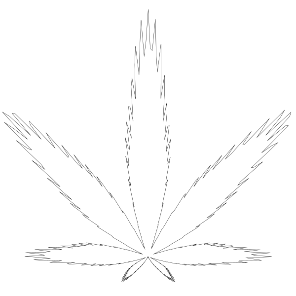
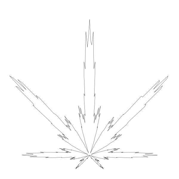
That gives me this image:
Ah, OK. This tells us a few things.
First, this formula is using Cartesian coordinates and I’m using upside-down screen coordinates. So I’ll have to flip the y-axis. No problem.
Next, the center is where all the “leaves” join. So after flipping, I can probably set the center more towards the bottom of the canvas.
Finally, I guessed that 140 would be a good value for radius, as it would keep it well within the 600×600 size of the canvas. In fact, I expected it would only be about half the size of the canvas. But we actually go well beyond the canvas edge for the larger leaves. We could correct that in the code, maybe multiplying radius by some fraction to bring the largest leaf down to the radius the user passed in. I’m going to skip that part and just pass in a smaller value, but feel free to do what you want with the function.
Here’s my final version:
function cannabis(xc, yc, radius) {
  for (t = 0; t < 2 * PI; t += 0.01) {
    r = radius * (1 + 0.9 * cos(8 * t)) * (1 + 0.1 * cos(24 * t)) * (0.9 + 0.1 * cos(200 * t)) * (1 + sin(t))
    x = cos(t) * r
    y = sin(t) * r
    lineTo(xc + x, yc - y)
  }
  closePath()
}
All I did was change the lineTo function to use yc - y instead of yc + y.
Then when I call it, I just change the parameters a bit (with a bit of trial and error to get it just right):
canvas(600, 600)
cannabis(300, 520, 120)
stroke()
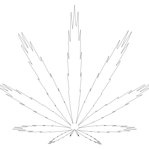
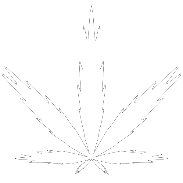
There we go!
Side note. I seriously considered changing the size of the canvas so that the yc parameter could be 420. You’ll either get that or you won’t. 🙂
Of course, now I’m curious about what that formula is doing. There’s basically four parts to it after the a, each in parentheses – three with cosines, one with sine. The first one has a hard coded 8 in there.
... (1 + 0.9 * cos(8 * t)) ...
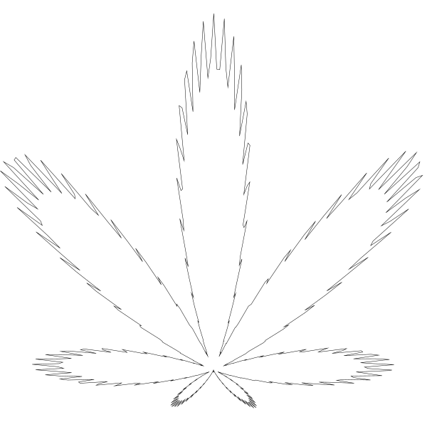
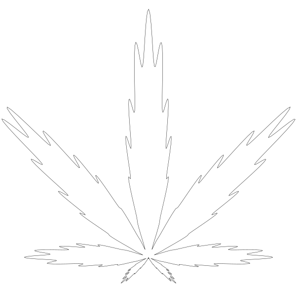
Since there are seven visible leaves there, I’m guessing those are related – there’s probably actually eight leaves, but the bottom one is too small to see. I’ll change that 8 to a 12…
Yup, theory validated. Eleven leaves plus an invisible one.
In the second section, the 24 is a bit less obvious.
... (1 + 0.1 * cos(24 * t)) ...
If I revert back to original and then change the 24 to 0, I get very rounded leaves.
Doubling 24 to 48 gives us:
It’s kind of making three levels for each leaf. Let’s put it back to 24 and change the multiplier:
... (0.7 + 0.3 * cos(24 * t)) ...
Again, we see three levels, which make sense, as 24 = 8 * 3. So this section is using a very small multiplier, 0.1, to make a subtle change to each leaf – making it just a bit less round. Cool. We’ll revert that and look at the next one.
... (0.9 + 0.1 * cos(200 * t)) ...
The 200 there makes me guess it’s creating all the jagged edges. If I change it to 100, it’s less jagged.
But now I’m seeing some blockiness. I can try increasing the resolution by changing the for loop increment from 0.01 to 0.005:
Mmmm… smooth.
I’ll revert that and look at the final sine block.
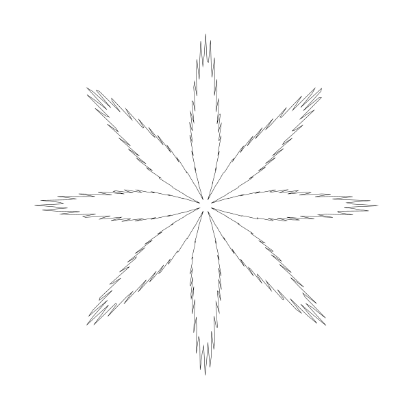
... (1 + sin(t))
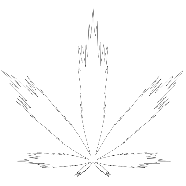
My guess was that this was affecting the orientation of the curve. I thought that if I removed that section, the leaf would be sideways. But I was wrong. Here’s what happens if I remove that section and set yc back to 300, the center of the canvas:
That was a pleasant surprise! And it gives me a lot of ideas of new curves I can create from this. Also, this makes that missing eighth leaf visible!
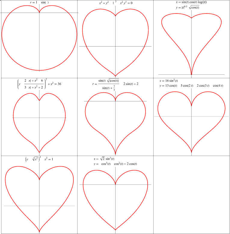
Again, Wolfram Mathworld to the rescue. As you can see, there is no single formula to draw a heart shaped curve. This page shows eight different ones. Personally I like the last one in the second row.
Rather than a polar formula like last time (and some of these other examples), this just has us computing the x and y directly. But we’re still going to loop a t value from 0 to 2 * PI.
For the y part of the formula, there are four different calculations. It’s not entirely clear how these calculations are supposed to be combined, but if you look further down in the text, you find that you’re supposed to subtract them. I’m also a bit concerned that we have so many hard coded numbers in there and no way to change the final size of the heart. But I’m sure we can figure that out.
Once again, this is really a pretty straightforward formula, so let’s jump in and code it up.
function heart(xc, yc) {
  for (t = 0; t < 2 * PI; t += 0.01) {
    x = 16 * pow(sin(t), 3)
    y = 13 * cos(t) - 5 * cos(2 * t) - 2 * cos(3 * t) - cos(4 * t)
    lineTo(xc + x, yc + y)
  }
  closePath()
}
We can run this like so:
canvas(600, 600)
heart(300, 300)
stroke()
And we’ll get:
Generally right, but we need to flip it like before, and we need to allow for changing the size. Right now it’s about 32 pixels wide. That’s the hard coded 16, times 2.
For flipping we can again just say yc - y.
For size, let’s first get rid of all of those hard-coded numbers by dividing them all by 16.
If we left it like that, we’d get a heart that would be two pixels wide (1 * 2). Now we can add a size parameter and multiply both values by that.
function heart(xc, yc, size) {
  for (t = 0; t < 2 * PI; t += 0.01) {
    x = size * pow(sin(t), 3)
    y = size * (0.8125 * cos(t) - 0.3125 * cos(2 * t) - 0.125 * cos(3 * t) - 0.0625 * cos(4 * t))
    lineTo(xc + x, yc - y)
  }
  closePath()
}
Now we call it like so:
canvas(600, 600)
heart(300, 300, 280)
stroke()
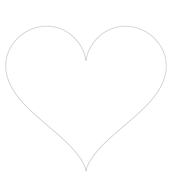
And get:
Not too difficult.
I’m not going to dive in to all the different ways you can mess with this, but just try changing the various constants in the formula and see what happens. Can you make it better? Come up with something completely different?
There are actually a truckload of different egg formulas on that page. Like the heart curve, I was surprised that there was no single standard egg curve formula.
But I homed in on the one on that page under the section “From the Oval to the Egg Shape”. This takes a general formula for an oval or ellipse and alters the “y radius” based on the current value at each point. If x is to the right of center, it will make the y value a little bit bigger. If x is to the left, it will make the y value a bit smaller. That seemed sensible.
So we’ll start with an ellipse formula. We covered that back in Chapter 3.
function ellipse(x, y, rx, ry) {
  res = 4.0 / max(rx, ry)
  for (t = 0; t < 2 * PI; t += res) {
    lineTo(x + cos(t) * rx, y + sin(t) * ry)
  }
  closePath()
}
That’s nice and concise, but I’m gonna break it up a bit so we can mess with the raw x and y coords right out of the trig functions before translating and scaling them. I’m also going to ignore the res variable and just hard code the 0.01 in there. Just for simplicity and clarity. Keep it if you want.
function egg(xc, yc, rx, ry) {
  for (t = 0; t < 2 * PI; t += 0.01) {
    x = cos(t)
    y = sin(t)
    lineTo(xc + x * rx, yc + y * ry)
  }
  closePath()
}
This will just draw an ellipse, but let’s make sure it works with the changes.
canvas(600, 600)
egg(300, 300, 280, 190)
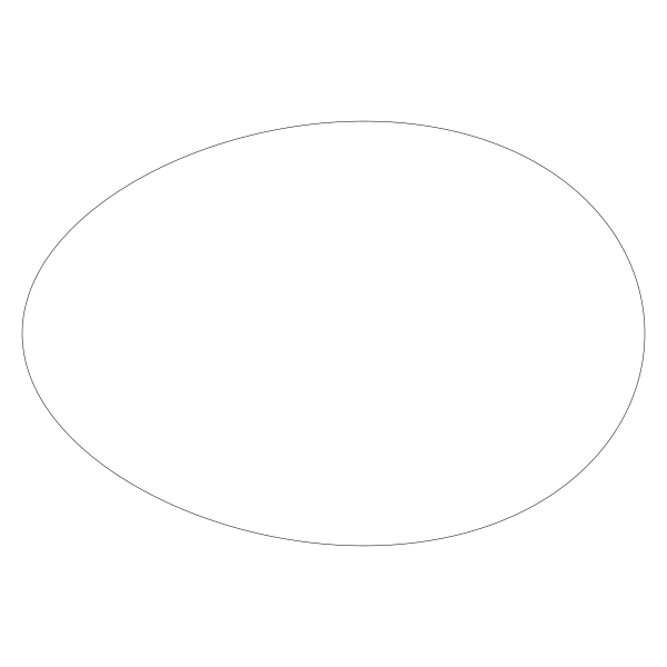
stroke()
Yup, that’s an ellipse. Where did I get the 280 and 190 from? Well, 280 is a bit less than half of the width of the canvas, so that’s the rx. And I wanted ry to be somewhat less than that. It was just trial and error and 190 looked about right.
Now let’s make this ellipse into an egg. The article gives three formulas:
Those t functions just give us something we need to multiply the y value by. I’m not going to make new functions though. I’m just going to do the multiplication right in the for loop. Let’s try the first one…
function egg(xc, yc, rx, ry) {
  for (t = 0; t < 2 * PI; t += 0.01) {
    x = cos(t)
    y = sin(t)
    y *= (1 + 0.2 * x)
    lineTo(xc + x * rx, yc + y * ry)
  }
  closePath()
}
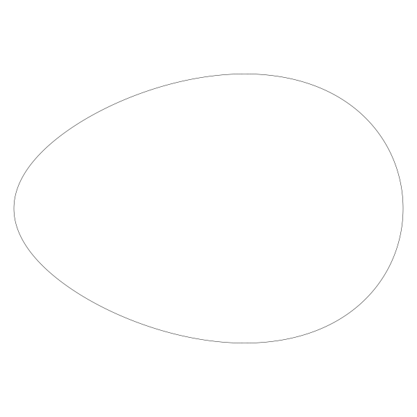
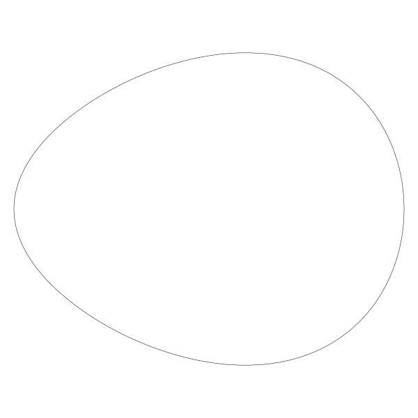
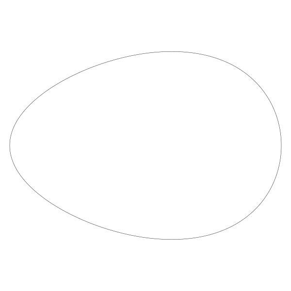
Woo! An egg!
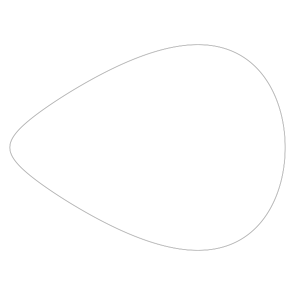
Now we can mess with that a bit. The 0.2 value there is probably going to be the best source of experimentation. Let’s try 0.3.
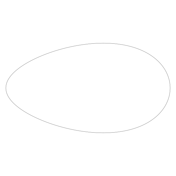
OK, it got a bit pointy. How about 0.5?
Even pointier. So we know where that’s going. Let’s go down. To 0.1.
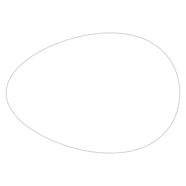
That’s barely distinguishable from the original ellipse. Which makes sense, because if that value was 0, than that line would do nothing and we’d be back to an ellipse. Let’s go back to 0.2, which probably did look the most egg-like, and try changing the yr value we’re passing in. We’ve been using 190. Here’s 220:
A nice fat egg. And 150:
I’m gonna stand by my choice of 190, but some minor tweaks might work better. Go for it. Let’s try the other formulas. We’ll go back to the ry of 190 first. Then change that line 5 to:
y *= 1 / (1 - 0.2*x)
This gives us:
And then the third formula:
y *= exp(0.2 * x)
Remember from Chapter 5 that most math libraries have an exp function that is e raised to a given power. That’s what we are doing here. The result of that:
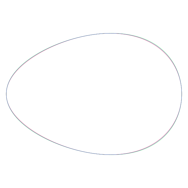
These all look suspiciously the same, so I drew them all at once, red, green and blue…
Yeah, those are all virtually the same. Maybe a pixel off here and there. Looking back at the original web site, they are talking about a different ellipse formula and multiplying y2 by that value:
The equation of the ellipse e.g. x²/9+y²/4=1 change to x²/9+y²/4*t(x)=1.
This is also hard coding 9 and 4 as divisors. If you unsquare those you get 3 and 2. And it just so happens that 2/3 of 280 is 186ish. So we pretty much agreed on my choice of 190 for ry!
At any rate, we have a formula that draws a fairly convincing egg no matter which algorithm we use. So I’m going to leave it there. Here I was literally writing the article as I was writing the code, so you really got to see my process, along with my glossing over of details in the source article. But it all came out just fine!
Summary
Hopefully this gives you some insight on how to find formulas in various places and convert them into code that draws something interesting – if you haven’t already done stuff like this.
And that wraps up this series on coding curves. At least for now. I have another series in mind though, so watch this space!