Chapter 6 of the Coding Curves Series

Another physical device which renders complex curves that we can simulate!

This one is called a Pintograph, and I’ve actually built one of these myself.

We’ll start with a video – this is literally the first video that came up when I searched Youtube for “pintograph”, but it does the job.

A pintograph can be considered to be a type of harmonograph, but rather than being based on pendulums, pintographs are usually driven by electric motors (though some are hand-cranked). There are disks attached to the motors and arms attached to the disks and a pen attached to the arms. You can change the size of the disks and where the arms are attached, the length of the arms and where they pivot, and the relative speed and offset of the motors to create a bunch of different types of curves.

For a long time I didn’t know where the word “pintograph” came from. I finally discovered it from the person who coined the term. Actually, their daughter coined the term. It comes from a pantograph, and the idea that the spinning wheels look like a Ford Pinto. Read more here: http://www.fxmtech.com/harmonog.html

In case you are not familiar with a pantograph, it’s a device that is often used for copying drawings. It has a few pivoting arms. You pin one of the pivot points so it doesn’t move, then put a pointer in one of the points and a pen in another. As you move the pointer along the original drawing, it moves the pen along the same shape. You can configure it to copy the drawing at the same size, or scale it up or down.

The Simulation

The pintograph we’ll simulate will be pretty simple. It will have two rotating disks with one arm attached to each. The arms will be attached to each other on the opposite end and that’s where the virtual pen will be.

First of all, we’ll need to simulate the two disks. They’ll each have an x, y position, a radius, a speed and a phase. We’ll make these visible to start with so you can get a feeling for what’s going on. Otherwise it would just be a long complicated formula.

We’ll create two circles and rotate them and show the point where the arms will be attached.

Each disk will be represented by this kind of structure:

disk: {
  x,
  y,
  radius,
  speed,
  phase,
}

Like last time, it doesn’t matter if this is a generic object, a struct, a class or what. I’m going to assume that you’ll also have a function that will create one of these disks like this:

d0 = disk(100, 200, 100, 2, 0.5)
d1 = disk(400, 200, 60, 3, 0.0)

Now we can set up an animation like so:

width = 600
height = 400
canvas = (width, height)
t = 0

d0 = disk(100, 200, 100, 2, 0.5)
d1 = disk(400, 200, 60, 3, 0.0)

function loop() {
  clearScreen()

  circle(d0.x, d0.y, d0.radius)
  stroke()
  x0 = circle.d0.x + cos(t * d0.speed + d0.phase) * d0.radius
  y0 = circle.d0.y + cos(t * d0.speed + d0.phase) * d0.radius
  circle(x0, y0, 4)
  fill()

  circle(d0.x, d0.y, d0.radius)
  stroke()
  x1 = circle.d1.x + cos(t * d1.speed + d1.phase) * d1.radius
  y1 = circle.d1.y + cos(t * d1.speed + d1.phase) * d1.radius
  circle(x1, y1, 4)
  fill()

  t += 0.1
}

Again, loop is a theoritical function that will be fun over and over again so that we get an animation. I’ve set mine up to create the frames for an animated gif, but this can be done as a real time animation as well. Here’s what I got:

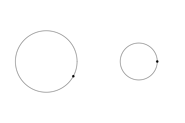
This doesn’t smoothly loop, but that’s ok. You can see that we have two disks of different sizes moving at different speeds. The code itself shouldn’t be too complex. We clear the screen and for each disk we draw a circle at its position and with its radius. Then we take an offset from that circle to calculate the point where the arm will be attached. This uses basic trig: x = cos(angle) * radius, y = sin(angle) * radius. Here, the angle is t times the disk’s speed, plus it’s phase. When we get that point, we fill a smaller circle there.

Attaching the Arms and Finding the Pen

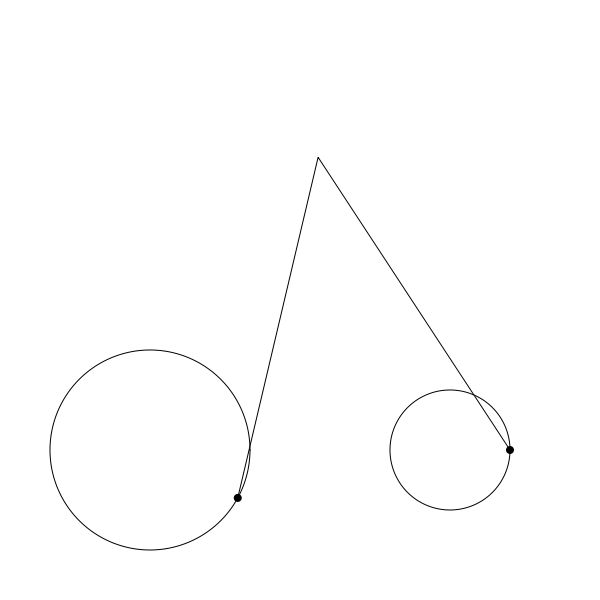
OK. Now things get a bit more mathy. We’re going to have two arms. each one is going to be attached to one of those spinning points at one and, and they’ll be attached to each other on the other end. At this point, a sketch is in order:

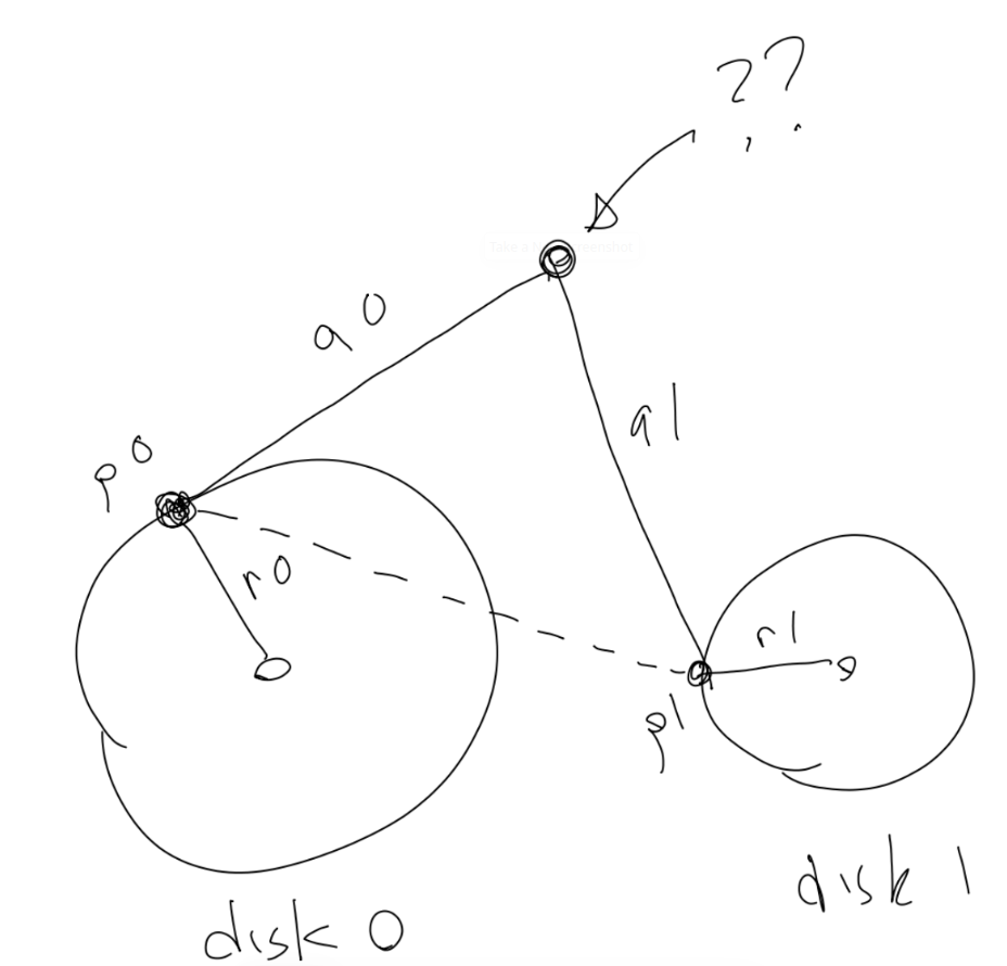
We have our two disks. Through their radii and rotation and position, we know the positions of points p0 and p1. That’s what we just did above. We can also define the lengths of those arms. They’ll be the same for now, but they could be different. We’ll call them a0 and a1. (I know, it looks like 90 and 91 in the sketch. Sorry!) What we need to do is get the position of that top point where the two arms join.

We can easily get the distance between p0 and p1 with the Pythagorean theorem. We can call that d. It’s represented by the dotted line in the diagram.

Now we have a triangle whose sides are a0, a1 and d.

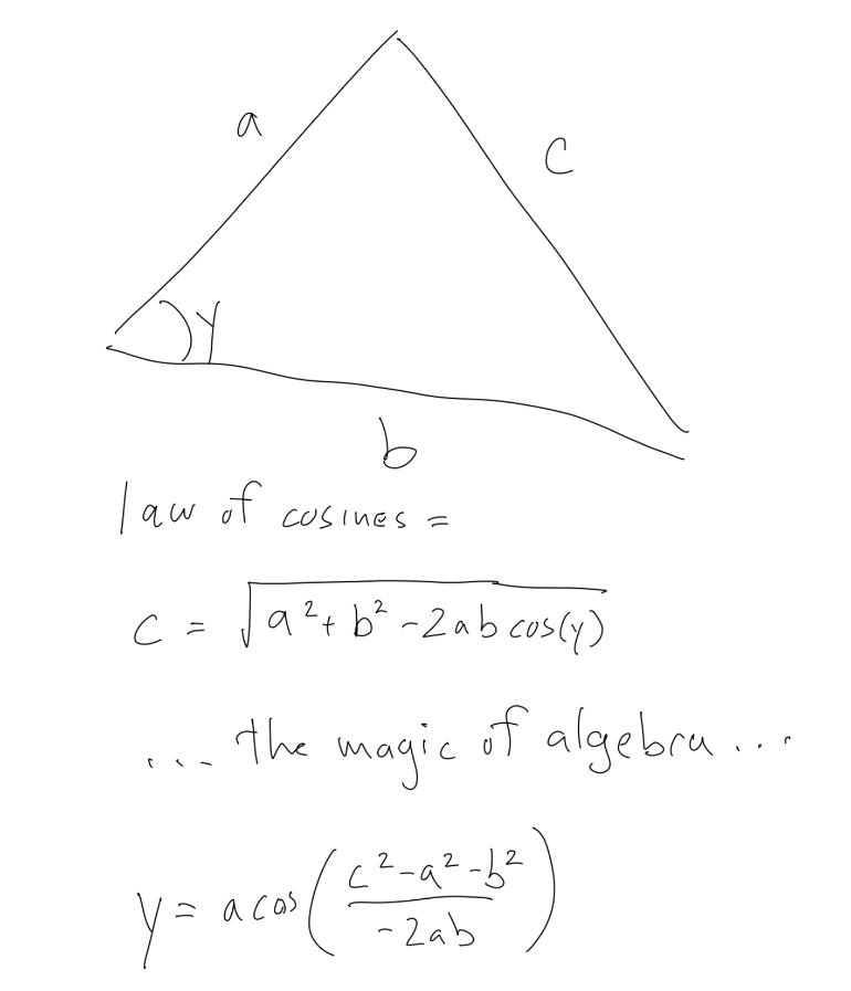
There’s a trigonometric rule called the “law of cosines” that will help us here. With it, if you you know the lengths of all three sides of a triangle, a, b, and c, you can get any angle of that triangle. Usually the way it’s written is as follows though:

c = sqrt(a*a + b*b - 2*a*b*cos(y))

… where y is the angle opposite side c. So if you know the length of two sides and the angle between them, you can find the length of the opposite side. Also useful in some cases, but not what we need here.

But we can rearrange that formula and put the unknown variable by itself on one side, and the other side will be the formula you need to calculate that value.

What I want is to know is one of those angles so I can use it to find the location of the pen. Here’s what I came up with, showing the formula, some hand-wavey algebra and the resulting formula we’ll need.

In our case, the sides we have correspond to the sides in the formula like so:

a = a0
b = d
c = a1

So if we apply this formula, we’ll get the angle between the p1, p0, and the pen.

We can also use atan2 to get the angle from p0 to p1. And if we subtract them, we get the actual angle that goes from p0 to the pen.

Again, a drawing is in order:

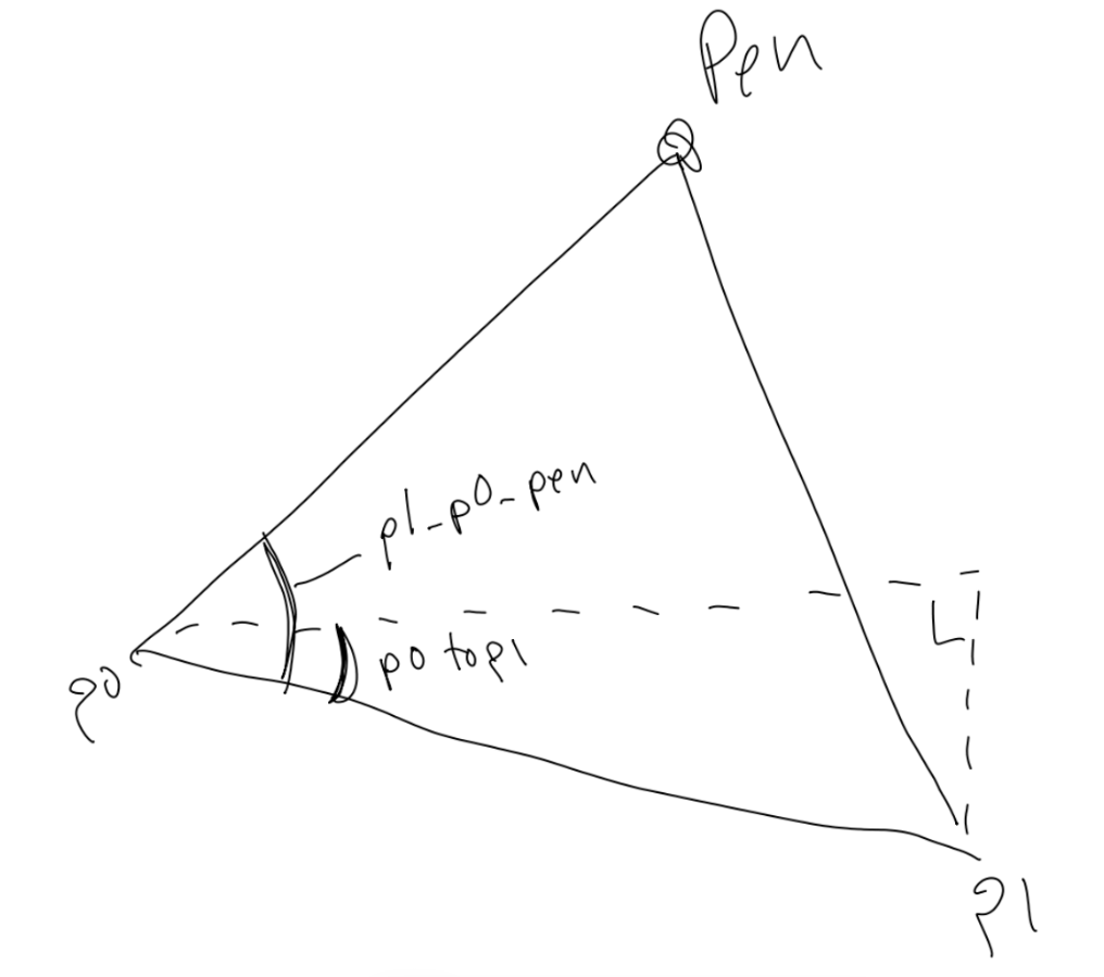
The big angle that goes from p1 to p0 to the pen, which we get with the law of cosines, we call p1_p0_pen. The smaller angle we get with atan2, we call p0toP1. Subtract them and we have the angle we have to go towards to get the location of the pen. I’m sure there are different ways to do this, and probably much better ones, but this one works. Once you have all the steps, you can further simplify it to something more concise, but I wanted to show the steps to hopefully have it make some sense.

Anyway, we can now code this up:

width = 600
height = 600
canvas = (width, height)
t = 0

d0 = disk(150, 450, 100, 2, 0.5)
d1 = disk(450, 450, 60, 3, 0.0)

function loop() {
  clearScreen()

  circle(d0.x, d0.y, d0.radius)
  stroke()
  x0 = d0.x + cos(t * d0.speed + d0.phase) * d0.radius
  y0 = d0.y + sin(t * d0.speed + d0.phase) * d0.radius
  circle(x0, y0, 4)
  fill()

  circle(d0.x, d0.y, d0.radius)
  stroke()
  x1 = d1.x + cos(t * d1.speed + d1.phase) * d1.radius
  y1 = d1.y + sin(t * d1.speed + d1.phase) * d1.radius
  circle(x1, y1, 4)
  fill()

  // the length of the arms
  a0 = 350
  a1 = 350

  // get the distance between p0 and p1
  dx = x1 - x0
  dy = y1 - y0
  d = sqrt(dx * dx + dy * dy)

  // find the two key angles and subtract them
  p1_p0_pen = acos((a1 * a1 - a0 * a0 - d * d) / (-2 * a0 * d))
  p0toP1 = atan2(y1 - y0, x1 - x0)
  angle = p0toP1 - p1_p0_pen

  // find the pen point
  pX = x0 + cos(angle) * a0
  pY = y0 + sin(angle) * a0
  
  // draw the arms
  moveTo(x0, y0)
  lineTo(pX, pY)
  lineTo(x1, y1)
  stroke()

  t += 0.1
}

With that, you should be able to render something like what you see below.

Again, this is a non-cleanly looping gif, but shows the idea at work. I’ve commented the code to explain what’s going on in each step. Hopefully that helps. Note that I also changed the size of the canvas and moved the disks towards the bottom to make room for the arms.

One thing to be careful of is making sure that the two arms are long enough so that they can always reach between the two connection points on the disks. In the real world, if they were too short, they’t probably just break or jam up the motors. In code, you’ll probably just get a NaN (not a number) error when you go to do the acos and you’ll be sitting there wondering what’s wrong. I speak from experience.

Drawing the Curve

Finally, let’s see what this thing draws. For this, I’m going to abandon the animation and stop drawing the circles and arms. I’ll just track where the pen is on each iteration and use that to draw a long, looping, Lissajous-ish curve.

width = 800
height = 600
canvas = (width, height)

function render() {
  t = 0
  
  d0 = disk(250, 550, 141, 2.741, 0.5)
  d1 = disk(650, 550, 190 0.793, 0.0)

  // the length of the arms
  a0 = 400
  a1 = 400
  
  for (i = 0; i < 50000; i++) {
    x0 = d0.x + cos(t * d0.speed + d0.phase) * d0.radius
    y0 = d0.y + sin(t * d0.speed + d0.phase) * d0.radius

    x1 = d1.x + cos(t * d1.speed + d1.phase) * d1.radius
    y1 = d1.y + sin(t * d1.speed + d1.phase) * d1.radius

    // get the distance between p0 and p1
    dx = x1 - x0
    dy = y1 - y0
    d = sqrt(dx * dx + dy * dy)

    // find the two key angles and subtract them
    p1_p0_pen = acos((a1 * a1 - a0 * a0 - d * d) / (-2 * a0 * d))
    p0toP1 = atan2(y1 - y0, x1 - x0)
    angle = p0toP1 - p1_p0_pen

    // find the pen point
    pX = x0 + cos(angle) * a0
    pY = y0 + sin(angle) * a0
  
    lineTo(pX, pY)
    t += 0.01
  }
  stroke()
}

I’ve left lots of room for you to optimize this, so go for it! Even in its rough form though, this code should draw something like this:

There’s lots of things to play around and experiment with here. But the truth is that this is a pretty simple pintograph, so mostly the shapes are going roughly look like what you see above. But you can build on these principles and make all kinds of more complex devices. This site has several demos to inspire you:

https://michaldudak.github.io/pintograph/demo/

Disks on disks, and rotary pintographs and 3-wheel pintographs, etc.

And if you’re into this stuff, just search “harmonograph”, “pintograph” and “drawing machines” on Youtube to get an endless supply of inspiration – either for coding or actually building. Some of the more interesting ones (in my mind) are the ones that draw the curves on a piece of paper that itself is slowing rotating on a turntable.

Summary

This wraps up our discussion of Lissajous curves and the simulation of physical drawing machines. At least for a while. Next time we’ll go back a bit more to basic, standard geometric curves.