Chapter 5 of the Coding Curves Series

This installment builds on Chapter 4’s discussion of Lissajous curves. Actually, a harmonograph is not a type of curve, it’s a device used to draw Lissajous (and similar) curves. And when I say a device, I mean a real world physical device that has ropes or chains and levers and pen and paper or bottles of sand and pendulums or other mechanics to create these curves.

Real Harmonographs

The first time I saw a harmonograph was at the Museum of Science in Boston on one of my many childhood trips there. It was a pendulum with a container of sand that leaked out and created a trail. The video below is not the exact one I was familiar with, but is essentially the same thing. I didn’t know it was called a harmonograph until many years later.

The video is worth watching and discusses Lissajous patterns in depth. With a pendulum, the time it takes to go back and forth is called its period, but it’s what we called the frequency in the last installment of this series. At around 4:12 in the video, the presenter explains how this pendulum can have two different periods – one on each axis. This is why the patterns it forms look like Lissajous curves – because they are! If each axis had the same period, it would just create circles and ovals and spirals. Still technically Lissajous curves, but not as interesting.

Here’s another version using a pen and paper:

In this case, the pen is stationary and it’s the paper that moves around on a pendulum. But it accomplishes the same thing.

Here’s another video of a similar setup, which appears to be made of cardboard, string and tape!

There is a key difference between a pure Lissajous curve and a mechanical, pendulum-based harmonograph though. The pendulum slowly loses energy and the distance it travels on each pass gets smaller and smaller. Eventually it will stop swinging all together and sit stationary in the middle of the drawing.

While this type of harmonograph will produce some interesting drawings, you can make it even more complex by using a double pendulum. A common way to do this is to have the paper or drawing surface moving on one pendulum, and the pen moving on another one.

Here’s one example of this:

Here, both the paper and pen are mounted on top of the pendulums, which are weights swinging below the table. So they move independently and are able to produce more complex curves.

And here’s yet another video of a very fancy double-pendulum, showing some of the amazing drawings it can create. Quite a couple of characters here too.

Simulated Harmonographs

As this is more of a programming focused site, I’m not going to explain how to build a physical harmonograph. But, these devices operate on the principles of physics. And the formulas that control them are known. We can use these formulas to create a virtual harmonograph.

We’ll start with a simple, single pendulum version. But first, let’s revisit our Lissajous curve formula:

x = A * sin(a * t + d)
y = B * sin(b * t)

A and B are the amplitude of the wave on each axis and a and b are the frequencies. And d is the delta, which puts x out of phase with y. And of course t is the parametric time variable. Initially we said that t would go from 0 to 2 * PI, but later we saw how it could increase infinitely.

To start to move towards simulating a harmonograph, we’ll recognize that each axis will have its own phase, rather than thinking one is phased and the other … unphased? So we’ll change the single d to p1 and p2.

x = A * sin(a * t + p1)
y = B * sin(b * t + p2)

This still gives us a Lissajous curve, but with a bit more complex definition. To fully move it to a simulated harmonograph, we’ll need to simulate that loss of energy, or damping. To do this fairly accurately, this will be an additional multiplier that looks like this:

e-d*t

… or “e to the power of minus d times t”

In code, that might be:

pow(e, -d * t)

Where pow is the power function, available in any fine math library.

So what is all this? We have two new variables here: e and d. Actually e is a constant, aka Euler’s number, equal to approximately 2.71828. I’ll let you read up on that on your own, but e is used in all kinds of real world physical formulas. Including, it seems, the damping of pendulums.

By now you might have guessed that d is for the damping factor. We’ll set d to a pretty small number, something like 0.002 is good to start with. Now when t is 0, that will make the exponent 0 and the result of the power calculation will be 1.0.

As t increases, by say 0.01 on each iteration, the value of the exponent will slowly grow negatively. When t is 0.01, the exponent will be -0.00002, and the result of the whole damping equation will be 0.9999800002.

After 100 iterations, t will hit 1.0 and the damping factor will be 0.9980019987. After 1000 iterations, it will be 0.9801986733. So you can see this goes down very slowly. If you increase d, it adds more damping and that number will go towards 0.0 faster. Here’s how we work it into the harmonograph equation:

x = A * sin(a * t + p1) * pow(e, -d1 * t)
y = B * sin(b * t + p2) * pow(e, -d2 * t)

Notice I made it d1 and d2, so you can have separate amplitudes, frequencies, phases and damping for each axis.

To bring it all home, as t increases, that last part of the equation moves closer and closer to 0.0, meaning both x and y will get smaller and smaller and will eventually be 0.0 themselves, simulating the pendulum running down and stopping. The higher d1 and d2 are, the quicker that will happen.

Depending on the math library you use, there may be a shortcut here. Since taking e to some power is a pretty common operation, there’s usually a built in function for doing just that, often called exp. For example in JavaScript, you could say Math.exp(-d1 * t), which would be exactly the same thing as Math.pow(Math.E, -d1 * t), but a bit shorter, and potentially more optimized.

Thus we can change the pseudocode to:

x = A * sin(a * t + p1) * exp(-d1 * t)
y = B * sin(b * t + p2) * exp(-d2 * t)

The Function

Let’s make something happen! Here’s our function:

function harmonograph(cx, cy, A, B, a, b, p1, p2, d1, d2, iter) {
  res = 0.01
  t = 0.0
  for (i = 0; t < iter; i += res) {
    x = cx + sin(a * t + p1) * A * exp(-d1 * t)
    y = cy + sin(b * t + p2) * B * exp(-d2 * t)
    lineTo(x, y)
    t += res
  }
  stroke()
}

Whole lotta parameters goin’ on. But you should understand most of this by now. The one I’ll mention is iter. Earlier we were mostly looping from 0 to 2 * PI. Now we want to loop a whole lot more than that, as the curve is going to continue to change as it is dampened and the amount of motion decreases. We’ll use a very high number for iter which simulates the harmonograph running for a long time. Real world harmonographs can take five minutes or longer to complete a single drawing.

Here’s an example of the function in use:

width = 800
height = 800
canvas(width, height)

A = 390
B = 390
a = 2.0
b = 2.01
p1 = 0.3
p2 = 1.7
d1 = 0.001
d2 = 0.001
iter = 100000

harmonograph(width / 2, height / 2, A, B, a, b, p1, p2, d1, d2, iter)

Yeah… 100,000 – a hundred thousand iterations. Might take a second or two. But you should get something like:

Here are some others I came up with by trying random parameters:

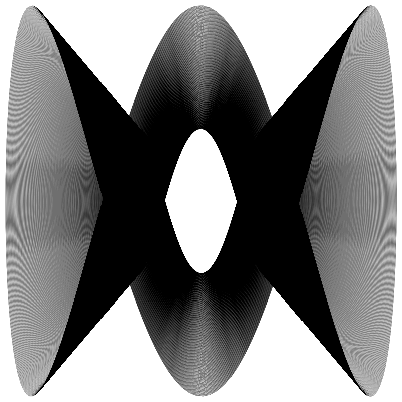
I’ve found that it’s best to keep a and b close to whole numbers, and let them vary by a very small amount, like in the first example where they were 2.0 and 2.01. It also works pretty well if the numbers are easily broken down into a relatively simple ratio, like 7.5 and 2.5 which is 3:1. And again, if you add a small amount to one of them it becomes a little more interesting, like 7.5 and 2.501. But totally random numbers like 5.7 and 3.2 will make for rather chaotic drawings.

The d values change how fast the pendulum is dampened, so a very low value will tend to draw more lines away from the center. Here’s the first example with damping on both axes at 0.0003:

And the same with damping of 0.003:

The pendulum decayed more quickly and you get more lines towards the center.

You can play with this endlessly. Try adding color too!

Double Pendulums

The drawings produced in that last video look pretty compelling. To do that, we need to come up with a double pendulum harmonograph simulation. You can consider that we have an x, y pendulum for the pen, and an x, y pendulum for the paper. Both will move independently, and wind up creating much more complex curves. You just need to calculate both x-axis pendulums and add them together for the final x, and the same on the y-axis.

Although the concept is relatively straightforward, this means we’ll be doubling the number of parameters we need.Four each for amplitude, frequency, phase and damping. If we do this naively, we might come up with something like this, which is really tough to manage.

// don't code this!!!
function harmonograph2(cx, cy, a1, a2, a3, a4, f1, f2, f3, f4, p1, p2, p3, p4, d1, d2, d3, d4, iter) {
  res = 0.01
  t = 0.0
  for (i = 0; t < iter; i += res) {
    x = cx + sin(f1 * t + p1) * a1 * exp(-d1 * t) + sin(f2 * t + p2) * a2 * exp(-d2 * t)
    y = cy + sin(f3 * t + p3) * a3 * exp(-d3 * t)+ sin(f4 * t + p4) * a4 * exp(-d4 * t)
    lineTo(x, y)
    t += res
  }
  stroke()
}

I’ve tried this and totally confused myself multiple times trying to remember which frequency value controlled which axis of which pendulum, etc. A better idea (maybe not the best, but better) would be to encapsulate the parameters needed for a single axis pendulum (amplitude, frequency, phase and damping) into a single value object, and pass four of those into the function.

I don’t know if the platform you’re using has classes or structs or plain old generic objects, so I’m just going to say that we have some kind of object with four properties:

pendulum: {
  amp,
  freq,
  phase,
  damp,
}

Don’t worry about the syntax here. Use whatever you need to use that will create such an object.

Now we can create four of these, maybe call them penX, penY, paperX, paperY. Like this:

penX = pendulum(90.0, 7.5, 1.57, 0.0001)
penY = pendulum(90.0, 4.0, 0.0, 0.0001)
paperX = pendulum(280.0, 1.001, 1.57, 0.0001)
paperY = pendulum(280.0, 2.0, 0.0, 0.0001)

Again, don’t get caught up in the syntax. This could be a factory function, a constructor, or you could just create some kind of object literal with those values – amplitude, frequency, phase and damp – for each pendulum.

Now we can change the harmonograph2 function to look like this:

function harmonograph2(cx, cy, penX, penY, papX, papY, iter) {
  res = 0.01
  t = 0.0
  for (i = 0; t < iter; i += res) {

    x = cx
      + sin(penX.freq * t + penX.phase) * penX.amp * exp(-penX.damp * t)
      + sin(papX.freq * t + papX.phase) * papX.amp * exp(-papX.damp * t)

    y = cy 
      + sin(penY.freq * t + penY.phase) * penY.amp * exp(-penY.damp * t)
      + sin(papY.freq * t + papY.phase) * papY.amp * exp(-papY.damp * t)

    lineTo(x, y)
    t += res
  }
  stroke()
}

There’s still a lot of code duplication there, but at least the method signature is better. I’ve done what I could to make it as readable as possible. There’s probably more you can do to make this whole set up easier, but that’s often the fun part of programming something complex – taking a somewhat janky proof of concept and turning it into an elegantly coded application. I don’t want to take that away from you, so I’ll leave plenty of room for improvement.

Anyway, now you can take those pendulum values we created and feed them into the function like so:

penX = pendulum(90.0, 7.5, 1.57, 0.0001)
penY = pendulum(90.0, 4.0, 0.0, 0.0001)
paperX = pendulum(280.0, 1.001, 1.57, 0.0001)
paperY = pendulum(280.0, 2.0, 0.0, 0.0001)

harmonograph2(width/2, height/2, penX, penY, paperX, paperY, 100000)

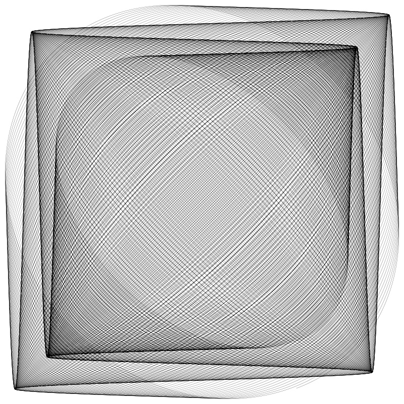
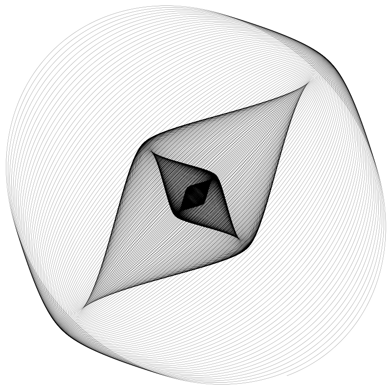
And if you’ve done everything right (and if I wrote this all up correctly), you should get an image like this:

penX = pendulum(50.0, 17.5, 1.57, 0.0001)
penY = pendulum(50.0, 11.0, 0.5, 0.0001)
paperX = pendulum(280.0, 0.50, 1.57, 0.0007)
paperY = pendulum(280.0, 1.50, 0.0, 0.0007)

Anyway, play with that for a while. There is an infinity of shapes you can create.

Animation

So far, we’ve just created static images here, but this is ripe for animation. You can do the obvious and show the curve building up over time just as if a real harmonograph were drawing it. I’ll skip over that one as it’s pretty easy and from my viewpoint not all that interesting.

What’s more fun is to animate some of the other properties. The phases are good candidates. Here’s an example where one of the phase values just moves from 0 to 2 * PI. It almost looks three-dimensional.

And here, some of the damp values are going back and forth between 0.001 and 0.0001.

Summary

So that’s harmonographs. Code it up and have some fun with it. There’s an endless ways you can tweak this to create interesting shapes. Heck, you might even decide to go buy some hardware and make a physical harmonograph. I’d love to see it if you do.

Next chapter we’ll be looking at yet another physical device and simulating that.