Chapter 3 in the Coding Curves Series

In this installment we’ll look at how to draw arcs, circles and ellipses. (And wander off on some tangents before we get done.)

It’s likely that your platform’s drawing api has at least some of this built in. For example, the HTML Canvas api does not have a circle method, but it does have an arc method as well as an ellipse method, either of which can be used to draw circles.

But it’s good to know how to do all of these manually. You’ll wind up using it someday, somewhere on some platform.

First let’s just look at arcs and circles. You can say that an arc is just part of a circle, or you could say that a circle is an arc that extends 360 degrees. So we could go at this either direction, but it makes sense to me to start with circles and specialize into arcs.

Note on Measurements

The drawing api I am using has the y-axis reversed from standard Cartesian coordinates. Negative values go up, positive down. This is very common for drawing apis which aren’t specifically made for math or science use cases. It’s the same with Processing, HTML canvas, Cairographics, .net graphics, and many others. Some apis do use Cartesian coordinates and have positive angles going counter-clockwise. Yet others, such as pygame, mix the systems – y values go down positively, but positive angles go couter-clockwise.

This affects the measurements of angles. Zero degrees is due east. In a Cartesian system, positive angles will move in a counter-clockwise direction and negative angles in a clockwise direction. In reversed y-axis systems, the opposite is true. In this chapter, I don’t make any attempt to “correct” this. The functions we’ll be creating here will mirror the built-in functions of many drawing apis.

But know that if you do want to create circle, arc and ellipse functions that operate per the Cartesian coordinates, that’s easy enough to do. And when you finish the section on arc, you’ll know how to do that.

Circles

Definition

A circle is usually defined something like “the set of points that are equidistant from a given center point”. But when you are trying to draw a specific circle, that’s not very useful. I don’t need a set of infinite points. I just need enough points to draw short line segments through that will form a circle.

You’ll also see the “equation of a circle” as x2 + y2 = r2. Also pretty useless from the perspective of trying to draw one.

But then you get to the parametric form:

x = a + r * cos(t)
y = b + r * sin(t)

Here, a, b is the center of the circle, r is the radius, and t is a parametric variable that ranges from 0 to 2 * PI.

This starts to get useful. We can define the center point and the radius and then run a for loop from 0 to 2 * PI to get a set of points that we can draw lines through.

Eternal reminder. All the code here is pseudocode. See the first post in this series for more info.

width = 600
height = 600
canvas(width, height)

cx = width / 2
cy = height / 2
radius = 250
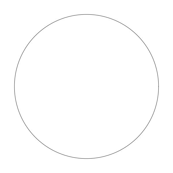
for (t = 0; t < PI * 2; t += 0.01) {
  lineTo(cx + cos(t) * radius, cy + sin(t) * radius)
}
closePath()
stroke()

Depending on your drawing api, you might need to start off with a moveTo before the lineTos. If so, I trust you’ll figure that out. Otherwise, this is straightforward. cx, cy and radius are a, b and r from the above formula. And t is the angle we loop through.

Note the final closePath call there. That’s a feature of most drawing apis. It will draw a final line segment from where the last operation left off to the place where the current path started, closing the circle. It might be different on your platform but there should be something there.

This gives us…

One question is the 0.01 value in the for loop. At this point, this was just a rough guess. If you make it too big, like 0.2, then you’re going to be jumping around the circle in large jumps and it’s not going to look quite as good:

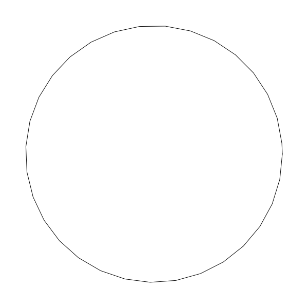
But if you make the increment too small, then you’re doing a lot of extra work for nothing. The larger the radius, the larger the circumference, and the more segments you need to use to make it smooth. The smaller the radius, the fewer the segments you need.

If you’re going with a constant 0.01 increment, you’re drawing 628 segments for each circle. This is way too many for a small circle.

By shear trial and error, I’ve found that a workable resolution seems to be about 4.0/radius. This looks good on circles down to a radius of 5. And on a radius of 200 draws half as many line segments as an increment of 0.01 and looks just as good. You can do some experiments on your own and see what looks good to you as it may vary by system.

A Function

With this, we can make a circle drawing function like so:

function circle(x, y, r) {
  res = 4 / r
  for (t = 0; t < PI * 2; t += res) {
    lineTo(x + cos(t) * r, y + sin(t) *r)
  }
  closePath()
}

Note that I left off the stroke in the function. This way you can create the circle with this function and then choose to stroke it, fill it or do both. If you want, you can make a strokeCircle function and a fillCircle function. Here’s how you’d use this:

width = 600
height = 600
canvas(width, height)

circle(width / 2, height / 2, 200)
stroke()

Arcs

Now that we have that down, we can build on this to create an arc function. Again, your api may already have this, but lets’ do it anyway.

This’ll be pretty easy. It’s the same as the circle function, but instead of starting at 0 and ending at 2 * PI, we let the user say what angles they want to start and end at.

This is all pretty straightforward, I’ll just throw the code out here without any pre-explanation:

function arc(x, y, r, start, end) {
  res = 4 / r
  for (t = start; t < end; t += res) {
    lineTo(x + cos(t) * r, y + sin(t) *r)
  }
  lineTo(x + cos(end) * r, y + sin(end) *r)
}

Told you it was simple. Instead of hard-coding the start and end angles to 0 and 2 * PI, we make them parameters. Also, I removed the call to closePath and replaced it with a final lineTo that draws a last line to the end angle, just to be precise.

To use it:

width = 600
height = 600
canvas(width, height)

arc(width / 2, height / 2, 250, 0.5, 3.5)
stroke()

And that gives you:

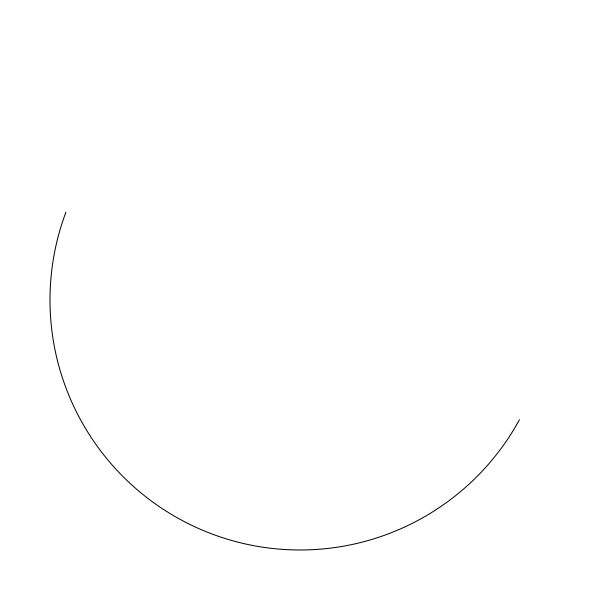
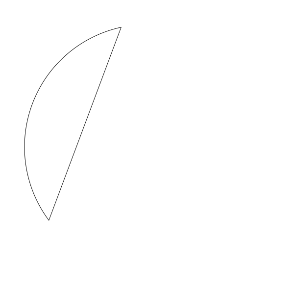
But there are a couple of problems. What if I entered the start and end angles in the opposite order?

arc(width / 2, height / 2, 250, 3.5, 0.5)

This will jump out of the for loop right away because 3.5 is already greater than 0.5. Nothing gets drawn. What I probably wanted was to start at the angle of 3.5 and go around until I crossed the start of the circle and hit 0.5 again, like this:

One way to handle this is just to make sure that the end angle is greater than the start angle. We can do that by checking if it’s smaller and then adding 2 * PI to it until it is bigger.

function arc(x, y, r, start, end) {
  while (end < start) {
    end += 2 * PI
  }
  res = 4 / r
  for (t = start; t < end; t += res) {
    lineTo(x + cos(t) * r, y + sin(t) *r)
  }
  lineTo(x + cos(e) * r, y + sin(e) *r)
}

Now this should work as expected and produce the image shown above. One more thing though. We’re always making the assumption that we’re drawing the arc clockwise. We should allow the user to make that decision. Luckily this is pretty simple. We’ll just add another parameter, anticlockwise. If this is true, we just need to swap start and end and we should be good.

function arc(x, y, r, start, end, anticlockwise) {
  if (anticlockwise) {
    start, end = end, start
  }
  while (end < start) {
    end += 2 * PI
  }
  res = 4 / r
  for (t = start; t < end; t += res) {
    lineTo(x + cos(t) * r, y + sin(t) *r)
  }
  lineTo(x + cos(e) * r, y + sin(e) *r)
}

If you’re lucky, your language will let you do the swap like this:

start, end = end, start

If not, you’ll have to go the old fashioned route:

temp = start
start = end
end = temp

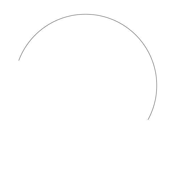
Now this code:

arc(width / 2, height / 2, 250, 3.5, 0.5, false)
stroke()

will give you this arc:

And this code:

arc(width / 2, height / 2, 250, 3.5, 0.5, true)
stroke()

will give you this arc:

Both start at an angle of 3.5 and draw an arc to 0.5. One goes one way, the other goes the opposite way.

As mentioned at the beginning of the article, positives angles going clockwise is the default I chose here, unlike Cartesian coordinates. Now that you know how to draw arcs in either direction, you are free to make your default whichever way you want.

Now that we have a solid arc function, we can actually go back and remove some duplication from our circle function, changing it to this:

function circle(x, y, r) {
  arc(x, y, r, 0, 2 * PI, true)
}

This draws an arc from 0 to 2 * PI, which is a circle.

Segments and Sectors

There are a couple of other functions you can create if you find them useful. A segment is an arc that is joined by a line segment between its beginning and end (a chord). We can do this by drawing an arc and then just calling closePath or whatever does that on your system.

function segment(x, y, r, start, end, anticlockwise) {
  arc(x, y, r, start, end, anticlockwise)
  closePath()
}

Here’s a segment that goes from an angle of 2.5 to 4.5:

And a sector is an arc that is joined by line segments that go to the center of the circle. We can do that by executing a lineTo to the center point and then calling closePath

function sector(x, y, r, start, end, anticlockwise) {
  arc(x, y, r, start, end, anticlockwise)
  lineTo(x, y)
  closePath()
}

Here is a sector drawn with the same angles as the segment example:

Now you’re well on you way to making pie charts!

Polygons

Before we move on to ellipses, I want to give you one bonus function: regular polygons. This isn’t what I would normally think of as a curve, but mathematically, it might be. Anyway, it’s low hanging fruit, right there for the picking, so let’s do it.

When we were talking about resolution, we saw how a low resolution circle starts to look chunky. You can see the individual line segments that make it up. Well, we can push that bug even further and turn it into a feature.If we push the resolution so low that we only wind up drawing six segments in our circle (exactly six), we have a hexagon. Five create a pentagon, four a square and three a triangle. We just have to specify how many sides we want, and divide 2 * PI by that number to get the resolution that will make that shape.

Here’s one take:

function polygon(x, y, radius, sides) {
  res = PI * 2 / sides
  for (i = 0; i < PI * 2; i+= res) {
    lineTo(x + cos(i) * radius, y + sin(i) * radius)
  }
  closePath()
}

Now you can call it like:

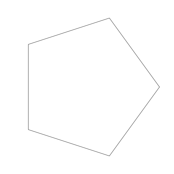
polygon(300, 300, 250, 5)
stroke()

and get a pentagon like this:

You might want to specify an initial rotation, you can do that like so:

function polygon(x, y, radius, sides, rotation) {
  res = PI * 2 / sides
  for (i = 0; i < PI * 2; i+= res) {
    lineTo(x + cos(i + rotation) * radius, y + sin(i + rotation) * radius)
  }
  closePath()
}

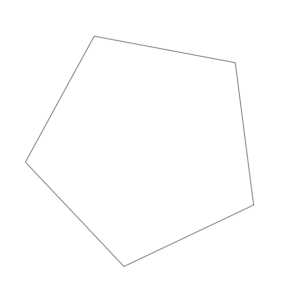
Now you can say

polygon(300, 300, 250, 5, 0.5)
stroke()

and have the polygon rotated a bit.

Try it with different numbers of sides.

A fun effect is to create a series of polygons of different sizes, each slightly rotated.

angle = 0
for (r = 5; r <= 255; r += 10) {
  polygon(300, 300, r, 5, angle)
  stroke()
  angle += 0.05
}

This creates a nice pattern like so:

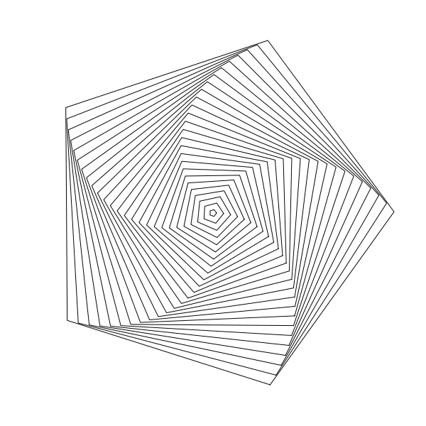
Might be a bit off-topic, but hey, there are five new emergent curves there! I’ll accept it.

Ellipses

Final bit of this installment, ellipses.

Well, let’s look at the definition of an ellipse, from Wikipedia…

a plane curve surrounding two focal points, such that for all points on the curve, the sum of the two distances to the focal points is a constant.

https://en.wikipedia.org/wiki/Ellipse

hmm… I get it, but doesn’t really help us to draw it. How about…

Ellipses are the closed type of conic section: a plane curve tracing the intersection of a cone with a plane

https://en.wikipedia.org/wiki/Ellipse

Nope. Let’s keep reading…

An ellipse may also be defined in terms of one focal point and a line outside the ellipse called the directrix: for all points on the ellipse, the ratio between the distance to the focus and the distance to the directrix is a constant.

https://en.wikipedia.org/wiki/Ellipse

OK, this is going nowhere. But as before, we can eventually find the parametric formula, which I’ve tweaked a bit to be similar to the one we had for the circle.

x = a + rx * cos(t)
y = b + ry * sin(t)

Here, in addition to the a and b that form the center position of the circle, we have rx and ry which I find easiest to think about as “radius x” and “radius y”, though these names will probably make mathematicians cringe. But for an un-rotated ellipse, rx will wind up being equal to half the ellipse’s width, and ry half its height.

So we can make a function:

function ellipse(x, y, rx, ry) {
  res = 4.0 / max(rx, ry)
  for (t = 0; t < 2 * PI; t += res) {
    lineTo(x + cos(t) * rx, y + sin(t) * ry)
  }
  closePath()
}

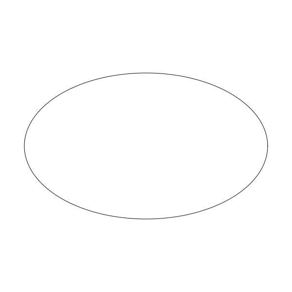
About the only thing worth mentioning here is that to get the resolution value, I divide 4.0 by the largest of the two “radii”. you might think of a better way, but this is good enough for me. Now you can call it like:

ellipse(300, 300, 250, 150)
stroke()

And get:

Bonus

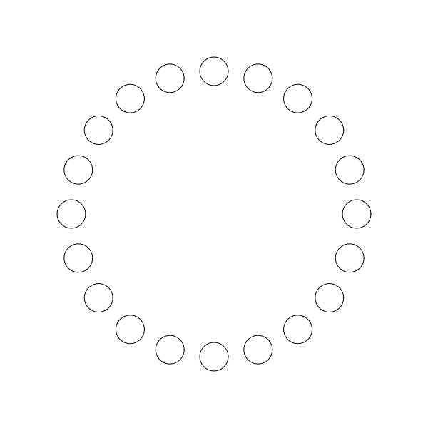
Sometimes I can’t stop writing. This next part isn’t really so much about creating curves… or maybe it is. You decide. But rather than draw line segments between each point on a circle (or arc, or polygon, or ellipse), we could just draw some other shape there. We’ll have to increase the interval that we use to draw the curve so all the shapes don’t mash together. In fact, the polygon method is perfect for this. This lets us draw a circle with a set number of circles. I’m not even going to explain this code. You should get it.

width = 600
height = 600
canvas(width, height)

cx = width / 2
cy = height / 2

res = PI * 2 / 20 // to draw 20 circles
for (t = 0; t < PI * 2; t += res) {
  x = cx + cos(t) * 200
  y = cy + sin(t) * 200
  circle(x, y, 20)
  stroke()
}

Which gives us:

Summary

I’m already elaborating on this in my head, but we’re off-topic enough, and this installment is long enough.

So far things have been pretty basic, but hopefully still interesting. From here on, they will get a bit more complex and hopefully even more interesting.