Chapter 2 in the Coding Curves Series

This is going to be a relatively simple one, but we’ll get into a few different applications. I’m not going to take a deep dive into what trigonometry is, there will be no images of triangles with the little square in the corner telling you which angle is 90°. No definitions of adjacent, opposite, hypotenuse. And NO soh-cah-toa!!!

I’m going to assume you know all that stuff. And if you don’t, a google search for basics of trigonometry will net you about 18,800,000 results in under one second. Proof:

So if you have no idea what I’m talking about in that first paragraph, stop here and do some learning on that stuff first.

Wait, what am I doing? Totally ignoring an opportunity for shameless self-promotion on my own blog. OK, here’s a playlist of trigonometry videos by myself. The best material on the subject out of all of those 18 million results, or your money back.

Coding Math – Trigonometry Playlist

But we have to start somewhere…

OK, there are a few basic trig functions that your language should have somewhere in it. Maybe they are global, maybe part of a math library. For this post, we’ll be dealing with what you’ll probably find named sin, cos, and tan. These stand for sine, cosine and tangent, which you should know about or have just learned more about above.

Let’s start with sin. You pass it a number and it gives you a number back. If you give it 0.0, it returns 0.0. As you increase that argument incrementally, the result you get will slowly increase up to 1.0 – or almost 1.0 anyway. Then as you continue to increase it it will go back down to 0.0, then down to -1.0 and back up to 0.0. As you continue to increase the argument, the result will continue to oscillate between -1.0 and 1.0.

Try it out:

for (i = 0.0; i < 6.28; i += 0.1) {
  print(sin(i))
}

In your language, you might need println or some kind of console or log function to display values. But you should get some output that looks like:

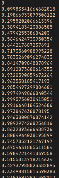
As I predicted, it starts at 0, goes up to 0.99957… and then starts going down again. Your output should continue going down to something like -0.999923… and then back up to almost 0.0.

Note that it did exactly one cycle of 0 to 1 to -1 to 0. Not a coincidence. It’s because the for loop ends at 6.28, which is approximately 2 * PI. Or 2 * 3.14… In most programming languages, the trig functions work on radians rather than degrees. This is another point I’ll assume you have some understanding of. But a radian is approximately 57 degrees. And 3.14… (PI) radians is 180 degrees. 6.28… (2*PI) radians is 360 degrees.

So the result of sin will go from 0 to 1 to -1 to 0 exactly one time from 0 to 360 degrees, or 0 to 6.28… radians.

If you change the for loop to end at PI (most languages have that as a constant somewhere) and the numbers should go from 0.0 up to 1.0, back to 0.0 and stop there. That’s half a cycle.

Bring on the Curves!

OK, let’s draw a sine wave. Size your drawing area to 800×500. It’ll also be helpful to set variables (or constants) to the width and height values. Then have a for loop with a variable x going from 0 to 800, using that width variable. Then we’ll take the sine of x and that will be our y value. We’ll add that to half the height so our sine wave will run along the center of the image. Draw a line segment to x, y and we’re all set.

Remember, this is all psuedocode. You’ll have to convert this to the language and drawing api of your choice. More details in the series intro.

width = 800
height = 500
canvas(width, height)

for (x = 0; x < width; x++) {
  y = height / 2 + sin(x)
  lineTo(x, y)
}
stroke()

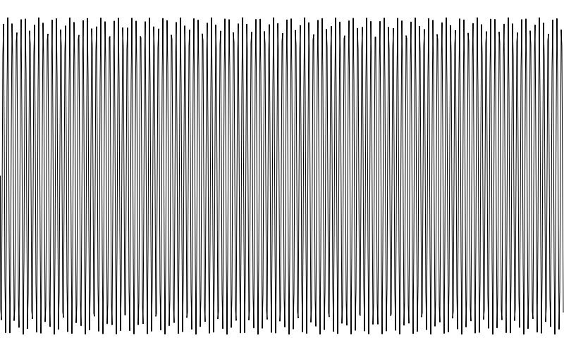
Depending on your drawing api, you might have to start with a moveTo(0, height/2) before you do the lineTos. When you’re done, you should have something like this image:

That’s a sine wave, but maybe not quite what you would expect. There are two problems, which is good, because they both lead into the next two things we need to talk about: wavelength/frequency and amplitude. Here, there are too many waves – the wavelength is too short (or the frequency is too high), and the waves themselves are mere blips – the amplitude is too low.

Amplitude

The amplitude is easy enough to handle. The sin function returns from -1.0 to 1.0, so we just need to multiply that number by an amplitude value and we’ll be good. The height times something like 0.45 will make the wave just smaller than the size of the canvas.

width = 800
height = 500
amplitude = height * 0.45
canvas(width, height)

for (x = 0; x < width; x++) {
  y = height / 2 + sin(x) * amplitude
  lineTo(x, y)
}
stroke()

That gives us height, but there are still too many waves so it’s hard to even comprehend this as a sine wave. We’ll fix that next.

Wavelength and Frequency

Wavelength is… wait for it… the length of a wave. Or the length between the same point on two consecutive waves. In the real world, these are actually physical distance measurements, with units anywhere from meters to nanometers, depending on what kind of wave it is you are measuring.

Another way of measuring waves is frequency – how many waves there are in a given interval (of space or time).

Wavelength and frequency are inversely related. A low wavelength (small distance between waves) equals a high frequency (many more waves in a given space). A high wavelength equals a low frequency.

You can write code to use either method of measurement. Let’s start with frequency.

Frequency

This is often specified as “cycles per second” (cps) rather than cycles in a given distance. Radio waves, for example, hit a receiver of some kind and we can just count how many hit it each second. The term “Hertz”, abbreviated “Hz” is the same as cycles per second. 100 Hz is 100 cycles per second. One kilohertz is 1000 cps, one megahertz is a million cps, etc.

Since we’re not dealing with moving waves though, it’ll be easier for us to measure frequency in terms of how many cycles occur in a given space. What you come up with here is up to your given application, but since we’re currently drawing a sine wave across an 800-pixel wide canvas, we can say that a frequency of one means that we should see one cycle occur as the wave goes across that canvas.

There’s a bit of math involved, so I’ll throw the pseudocode out there, then we’ll go through it.

width = 800
height = 500
amplitude = height * 0.45
freq = 1.0
canvas(width, height)

for (x = 0; x < width; x++) {
  y = height / 2 + sin(x / width * PI * 2 * freq) * amplitude
  lineTo(x, y)
}
stroke()

First we create a new variable, freq and set it to 1.0.

Then instead of just taking the sine of x, we divide x by width. This results in values from 0.0 to 1.0 as we move across the canvas.

Then we’ll multiply that by PI * 2. This will give us values from 0.0 to 6.28…, which should be familiar from the very first code example. This alone would make the results go from 0 to 1 to -1 and back to 0 exactly one time, as we saw. One cycle.

Finally, we multiply that by freq. That’s set to 1.0 now, so we’ll still get one cycle. With all this in place, you should be seeing this:

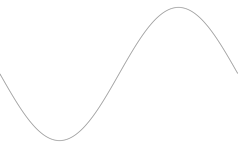
OK, that’s more like it. But you might be more used to the sine wave going up first, then down. If you’re seeing it go down and then up, like in my example, it’s because your drawing surface has the y-axis oriented such that positive values go down, the reverse of Cartesian coordinates. If you know how to use the 2d transform methods of your drawing api, you can fix it that way. I’ll go for a simpler fix of just subtracting y from height in the lineTo call.

width = 800
height = 500
amplitude = height * 0.45
freq = 1.0
canvas(width, height)

for (x = 0; x < width; x++) {
  y = height / 2 + sin(x / width * PI * 2 * freq) * amplitude
  lineTo(x, height - y)
}
stroke()

And now we have:

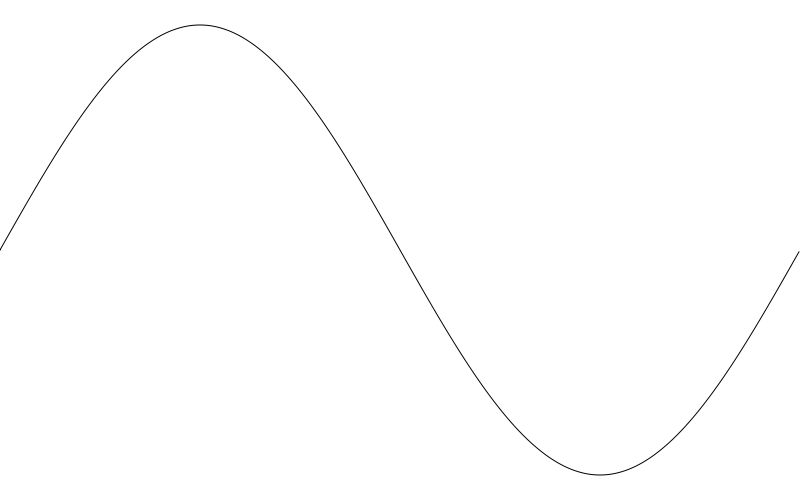
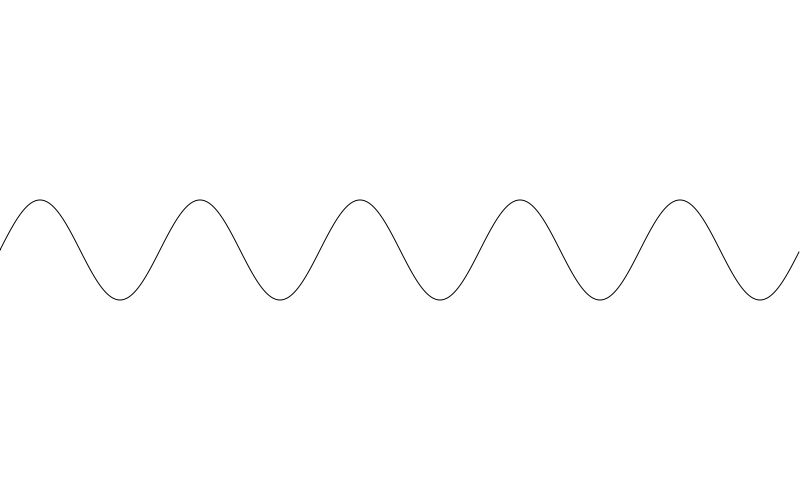
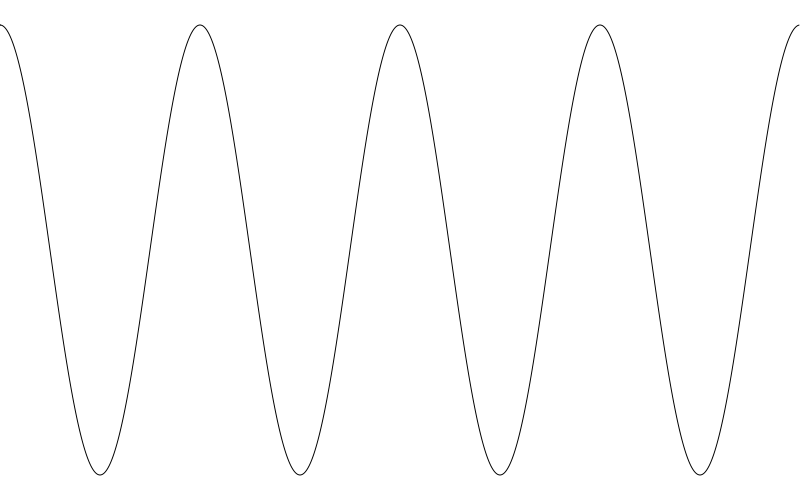
Now you can mess with those two variables, amplitude and freq to create different waves. Here I set amplitude to 50 and freq to 5:

Wavelength

Now let’s encode this to use wavelength instead of frequency. In this case we’ll be defining wavelength in terms of how many pixels it will take the wave to complete a full cycle. Let’s say we want one cycle to be 100 pixels long. Again, here’s the code, explanation to follow:

width = 800
height = 500
amplitude = height * 0.45
wavelength = 100
canvas(width, height)

for (x = 0; x < width; x++) {
  y = height / 2 + sin(x / wavelength * PI * 2) * amplitude
  lineTo(x, height - y)
}
stroke()

This time, inside the sin function call we divide x by wavelength. So for the first 100 pixels, we’ll get 0.0 to 1.0, then for the next 100 pixels 1.0 to 2.0, etc.

This gets multiplied by PI * 2, so for every 100 pixels we’ll get some multiple of 6.28… and will execute a complete wave cycle.

The result:

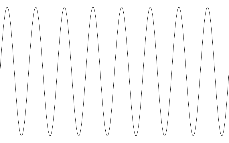
Since our canvas is 800px and the wavelength is 100px, we get eight full cycles, as expected.

Resolution

A quick word about resolution. Here, we are moving through the canvas in intervals of a single pixel per iteration, so our sine waves look pretty smooth. But it might be too much. If you are doing a lot of this and you want to limit the lines drawn, you can do so, with the possible loss of some resolution. We’ll just create a res variable and add that to x in the for loop and see what that does. We’ll start with a resolution of 10.

width = 800
height = 500
amplitude = height * 0.45
freq = 3
res = 10
canvas(width, height)

for (x = 0; x < width; x += res) {
  y = height / 2 + sin(x / width * PI * 2 * freq) * amplitude
  lineTo(x, height - y)
}
stroke()

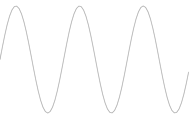
On the plus side, we are drawing only 10% of the lines we were drawing before. But you can already see that things have gotten a bit chunky. Going up to 20 for res reduces the lines drawn by half again. But now things are looking rough.

But the important thing is knowing the options, their benefits and tradeoffs.

Cosine

I’m going to keep this one really quick. Because everything I’ve said about sine holds true for cosine, except that the whole cycle is shifted over a bit. Going back to a single cycle and simply swapping out cos for sin …

width = 800
height = 500
amplitude = height * 0.45
freq = 1.0
canvas(width, height)

for (x = 0; x < width; x++) {
  y = height / 2 + cos(x / width * PI * 2 * freq) * amplitude
  lineTo(x, height - y)
}
stroke()

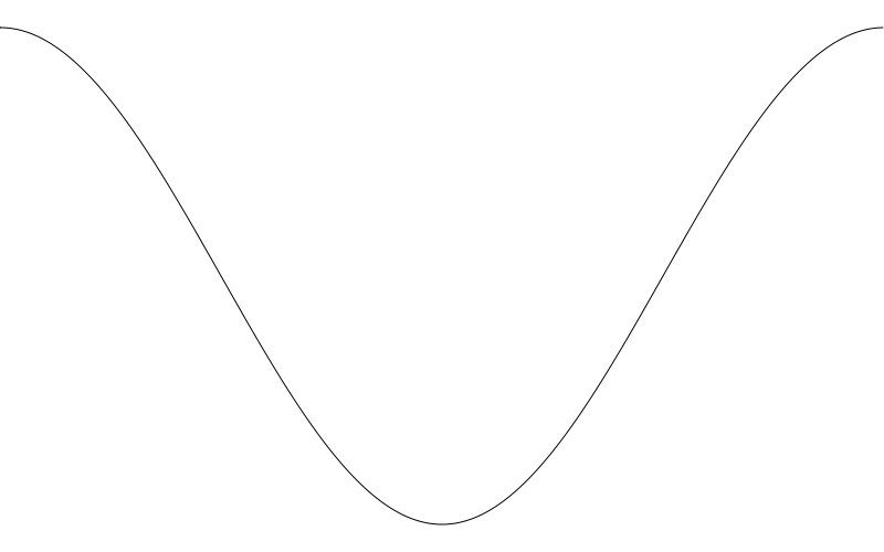
Here, an input of 0.0 gives us 1.0. And then we drop to 0.0, -1.0, back through 0.0 and end on 1.0 as we move from inputs of 0.0 to 2 * PI. It’s the same wave shifted over 90 degrees (or PI / 2 radians). It’s easier to see if we move the frequency up a bit.

I don’t really have a whole lot to say about cosine waves for this post. But we’ll be revisiting them again later in the series.

A Function

We can use everything we’ve covered so far to make a reusable function that draws a sine wave between two points. Again, I’ll do the pseudocode drop and then the explanation.

function sinewave(x0, y0, x1, y1, freq, amp) {
	dx = x1 - x0
	dy = y1 - y0
	dist = sqrt(dx*dx + dy*dy)
	angle = atan2(dy, dx)
	push()
	translate(x0, y0)
	rotate(angle)
	for (x = 0.0; x < dist; x++) {
		y = sin(x / dist * freq * PI * 2) * amp
		lineTo(x, -y)
	}
	stroke()
	pop()
}

This function has six parameters, the x and y coords of the start and end points, frequency and amplitude.

We get the distance between the two points on each axis as dx and dy.

Then, using these, we calculate the distance between the two points using the Pythagorean theorem and the sqrt function which should be somewhere in your language.

And we get the angle between the two points using the atan2 function that should also be available. If you don’t understand what’s happening so far, I suggest you go look at the references at the beginning of the post.

Now this function is assuming that your drawing api has some 2d transformation methods. If so, it probably also has a way to push and pop transforms from a stack. In HTML’s Canvas api for example, these would be context.save() and context.restore().

We want to push the current transform to the stack so we can transform the canvas, do our drawing, and then restore the earlier state when we are done. So we call push.

Then we translate to the first point and rotate to the angle we just calculated. At this point we just need to draw a sine wave using dist, freq and amp exactly as we’ve been doing.

Since our canvas is translated exactly as we want it, we can just call lineTo(x, -y) which just corrects the sine wave like we did before.

When we’re done, we stroke that path and call pop (or restore or whatever your api uses) to leave things how we found them.

We can now use this function like so:

width = 800
height = 500
canvas(width, height)

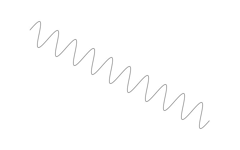
sinewave(100, 100, 700, 400, 10, 40)

This draws a sine wave starting at 100, 100, going to 700, 400, with a frequency of 10 and amplitude of 40.

If your drawing api does not have transform methods, I pity you. You can still do this kind of thing, but it will be much more complex. And beyond the scope of this post.

As mentioned in the comments below, the “frequency” aspect of this method might be a bit confusing, because the way it’s coded “frequency” means “number of cycles between point A and B”. So a long wave drawn with this method would have a larger wavelength than another, shorter line drawn with the same frequency. To address this, you might want to change the function to use wavelength instead. This would ensure that all waves drawn with the same wavelength would look similar, no matter how long they were. Another option would be to adopt a frame of reference for frequency, like “so many cycles per 1000 pixels” or something. What you do here depends on your needs and application, so I’ll leave that up to you.

Tangent

Drawing tangent curves is not nearly as useful as sine and cosine waves, but we’ll cover it for completeness.

Unlike the two functions we’ve covered so far, tangent does not constrain itself to the range of -1 to 1. In fact, it’s range is infinite. Let’s do the same thing we did for sin and just trace out the values.

for (i = 0.0; i < 6.28; i += 0.1) {
  print(tan(i))
}

You’ll get something like this:

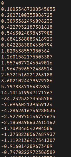
Again we start at 0, but quickly go up to 14, then jump to -34. But that’s deceiving. The values are truncated because we are moving in relatively large steps of 0.1. What is actually happening is that we are rapidly going up to positive infinity as the input angle approaches PI / 2 radians (or 90 degrees). Once it crosses that value, it jumps towards negative infinity, swiftly rises to 0.0 again at PI radians (180 degrees) and then repeats the cycle again once more before it gets to 2 * PI radians (360 degrees). This isn’t a linear progression though – it executes a curve as it approaches and leaves 0. Let’s code it up using frequency to see a single tangent wave cycle.

width = 800
height = 500
amplitude = 10
freq = 1.0
canvas(width, height)

for (x = 0; x < width; x++) {
  y = height / 2 + tan(x / width * PI * 2 * freq) * amplitude
  lineTo(x, height - y)
}
stroke()

Same thing here again, but swapped out tan for sin. I also reduced the amplitude just so we could see the curve better. In fact, it’s probably a misnomer to talk about the amplitude of a tangent wave since its amplitude is actually infinite. But this value does affect the shape of the curve.

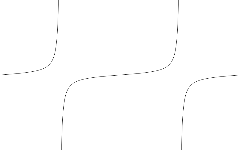
One thing to note is those near-vertical lines that shoot down from positive to negative infinity. Those aren’t technically part of the plot of the tangent. Mathematically, it implies that the tangent could have a value somewhere along that line at some point, but it will not. It is actually undefined at an angle of 90 and 270 degrees. And near infinity/negative infinity just before and after those values.

Not sure if this one will be of much use to you, but there it is.

Summary

Well, we got through the first few curves in this series. Good ones to have under the belt as a lot of other curves will uses these functions in one way or another. See you soon!