One of my tricks when coming up with new generative ideas is to take two (or three) completely unrelated techniques and combine them. I even created an app once where I had a long list of concepts and it would randomly combine them and come up with things like, “circle packing with diffuse limited aggregation”. (I just made that up and I’m not sure how it would work, but it’s intriguing, isn’t it?) I can’t say that the app ever sparked any projects that I ended up using, but I’ll probably go back to it some time and see if I can make it better.

This post was one of those successful combinations that evolved on its own and produced something that I have never seen anyone explore before. It produces a visualization of the forces behind a strange attractor that I find fascinating and beautiful. It feels like putting on special glasses that let you see the invisible workings of the universe.

Strange Attractors

I’ve been coding strange attractors for nearly two decades now. I’ve done them in Flash ActionScript, JavaScript, C#, Objective-C, Golang, Java/Processing and probably other languages. I’ve generated strange attractors as images, animated gifs, movies. I’ve created interactive apps to let the user explore attractors in real time, including a published iOS app. It’s one of my favorite techniques to explore and I always come back to it and try something new with it.

Background

The concept of a strange attractor is actually pretty simple, despite the complexity it winds up creating. I’ll stick to two dimensions here, but you can use the technique in three or more dimensions. You start with an x, y coordinate. You feed that into a function that returns a new coordinate. You do that a few hundred, thousand or even a few million times, plotting each point you get, and if you’re lucky you get a strange, looping shape.

There are many different strange attractor formulas. Each one has a number of constant parameters it uses on all iterations. Only the x, y coordinate changes. But because each iteration takes in the last coordinate as a variable parameter, a feedback loop is created. This results in one of a few possible behaviors:

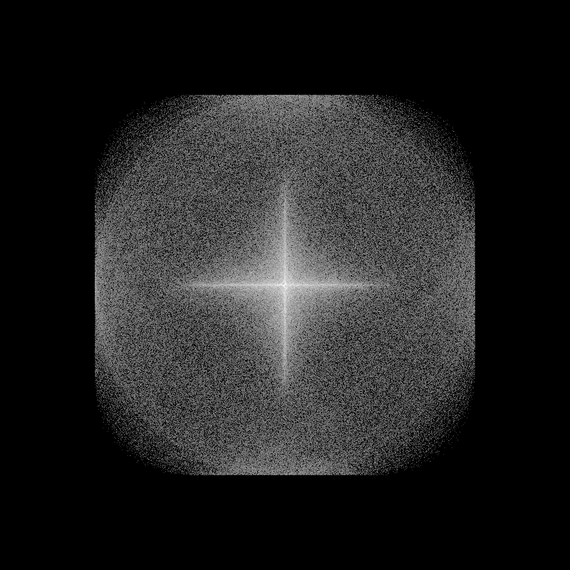
1. Chaos or nearly complete randomness. Not so interesting.
2. The successive points will converge on a small handful of locations. Not so interesting.
3. The points may diverge off to infinity. Not so interesting.
4. The points will loop around infinitely within a limited space, never following the exact pattern twice, but still adhering to a very complex pattern and forming one of these intricate, loopy shapes. Very interesting.

Here are a few examples showing chaos, convergence/divergence and looping.

From a strategy perspective, you might notice some similarity to the rendering of a Mandelbrot fractal. There, you are mapping each pixel to a point on the complex plane, iterating a function using that complex coordinate and checking to see whether it escapes to infinity or stays contained. Here, we are using a different formula, plotting each point and we’re usually only interested in those cases where the points do NOT escape into infinity.

An Example

It might be good at this point to look at some actual strange attractor formulas and their parameters. I’m not going to dive into any actual executable code in this post though.

I’ll show the attractor formula I’ll use for most of this post. This one is often referred to as the deJong attractor, created by Peter de Jong. One of the best places to get familiar with it is on Paul Bourke’s site.

Given an initial x, y pair, the formula is:

newx = sin(a y) - cos(b x)
newy = sin(c x) - cos(d y)

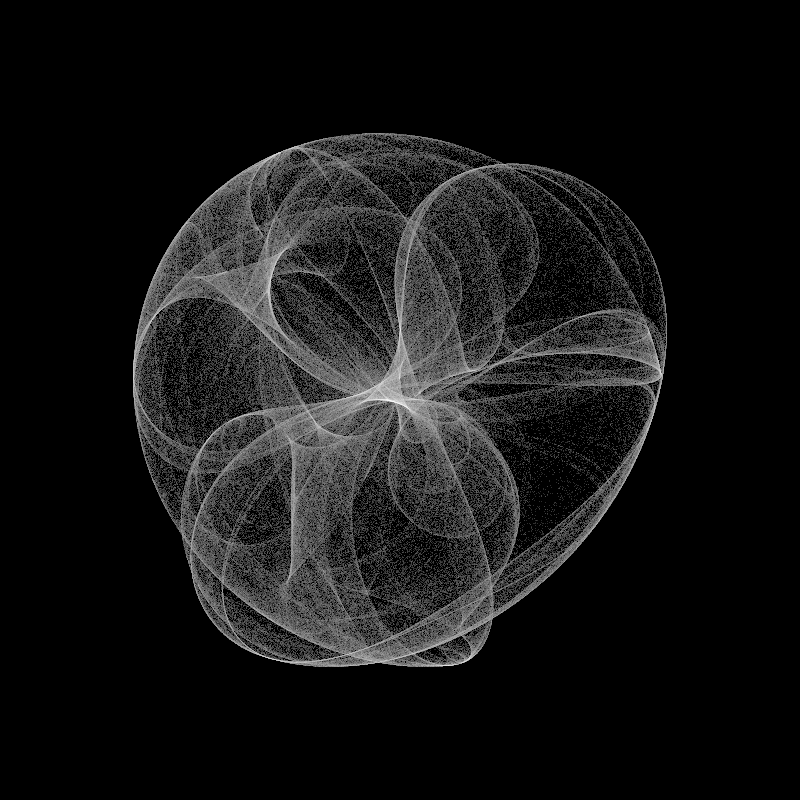
You’d then plot newx, newy and feed that back into the formula to get the next point and plot that. Repeat many thousands of times and you get something that looks like this:

Note that the values used by strange attractors are usually quite small. Usually well within the range of -10 to 10. Often much smaller even. So you’ll have to scale the points up into your image space before plotting them, or you’ll just get a tiny little splat. You’ll also want to transform your drawing space to put the origin somewhere in the center of your image, or everything will be stuck in the top left corner.

Also notice that in addition to the x, y coordinate, this formula has four constant parameters, a through d. By varying these, you get all kinds of interesting variations of shape and form, and also a whole lot of uninteresting garbage. Finding strange attractors is kind of a hunting expedition of changing the parameters until you find something you like by trying random parameters, then sneaking up on it until you have something just right. The above image was created with the constants set to the following (taken directly from one of Bourke’s examples):

a = 0.970
b = -1.899
c = 1.381
d = -1.506

Some Interesting Characteristics of Strange Attractors

Over the years I’ve learned various things about strange attractors that I find very interesting.

Starting point is irrelevant

One is that the starting point, what I’ll call the “seed” usually doesn’t matter at all. Depending on the formula, if you use zero for both x and y, that may cause it to collapse (not a problem in the deJong attractor). In general though, no matter what location you start with, you’ll still wind up in the same form, given the same constant parameters.

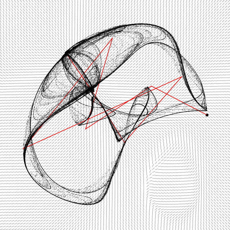
Honestly, I was not aware just how irrelevant the starting point is in many attractors. I had this idea that I would start with a number of different seed locations and color code each one and run some number of iterations using that color. My thought was that while they’d eventually converge on the main shape, there would be some number of iterations where each color would form a unique path. I was surprised to see how wrong this was, as you can see in this example:

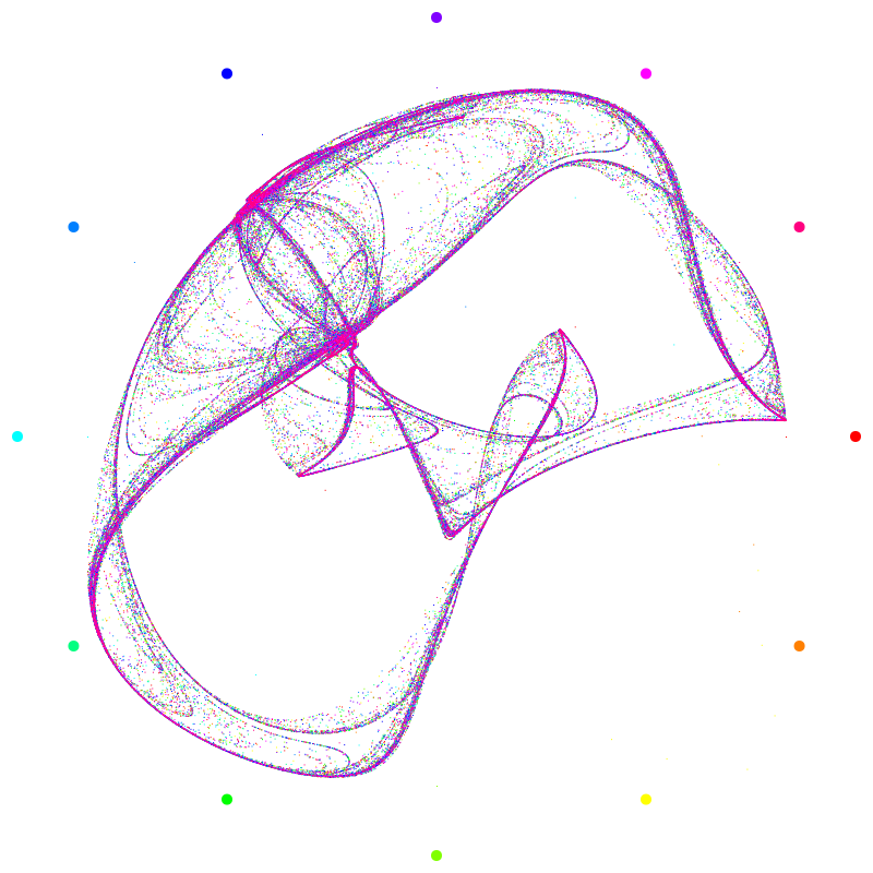
The larger colored dots are the seed locations. But it’s not like the colors in the shape are separated into distince areas or paths. It kind of appears that the maroon color hits certain areas harder, but those are just the most concentrated areas and that color is the last layer of color to go down so it just covers what was there before.

Note also that there is no discernible trace from the seeds to the shape itself.

This leads into my second observation:

The delta between points from consecutive iterations is large

You might see that cohesive form and expect that the points are wandering around it, moving in tiny steps like a particle simulation. That’s not the case though. Each consecutive point usually jumps almost completely across the shape to a new point quite far away. You can see that here:

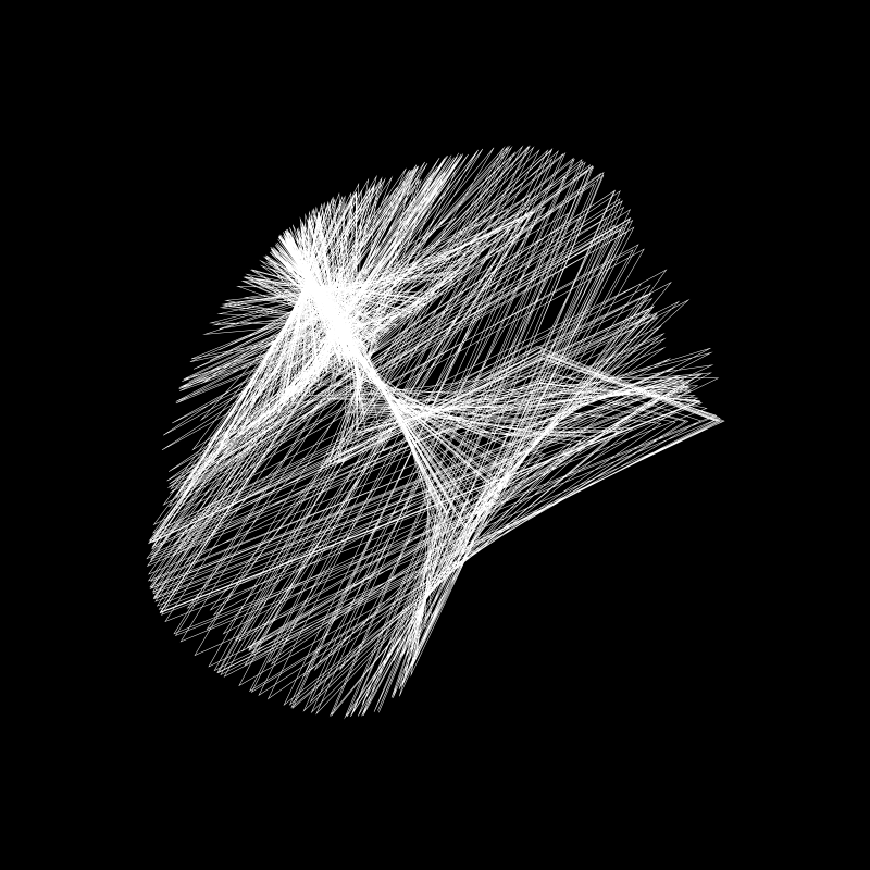
Here, I’ve mapped out 1000 iterations, connecting consecutive points with lines rather than just plotting them. The points almost seem to be ricocheting off of the inside of the shape. Given this behavior, it seems to me to be even more fascinating and unlikely that a cohesive shape would be formed. Yet it is.

This also explains why there is no discernible color trail in the earlier example. Even when the seed is well outside the shape, it jumps almost directly into range in the first few iterations in most cases.

On to Flow Fields

The above experiments got me thinking that for each point on the plane, there is a “force” pulling that coordinate to its next iteration. Calling it a force is probably a bit of a stretch, but there is a vector between any point on the plane and the next consecutive point. I realized this could be represented as a flow field.

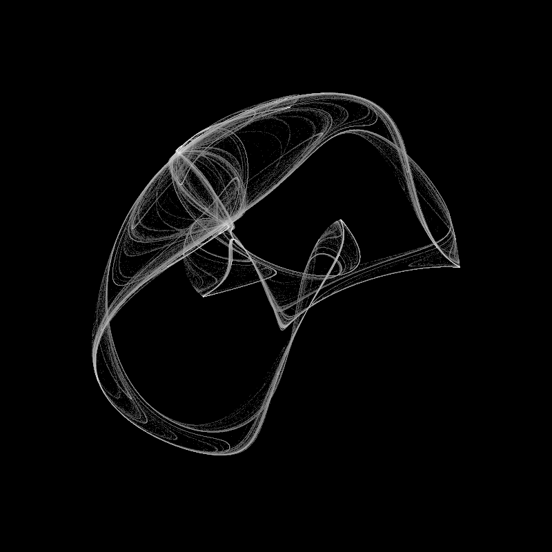
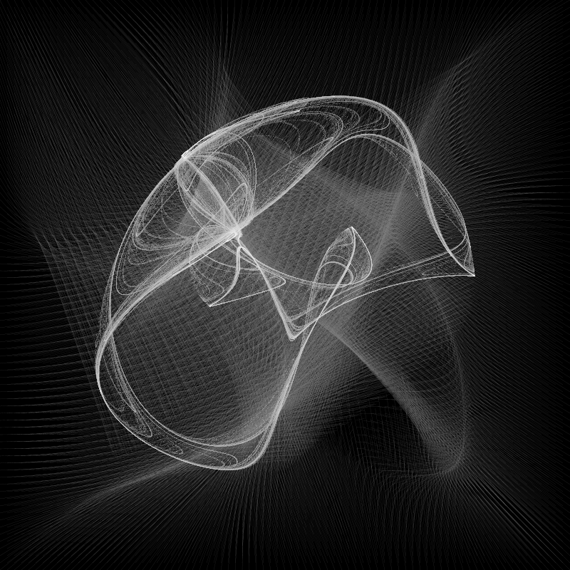
The strategy was to sample the plane as a grid of seed points and draw the “force” as a vector emanating from that seed location. Because the deltas are so large between each iteration, I first decided to represent only the direction of the vector at each point and use a unit length for magnitude. Here’s what that produced, overlaying the attractor result on top of the field.

This was pretty interesting. You can sort of see how the field contributes to the shape of the attractor’s form. What interested me most was that oval-shaped whorl in the lower right. It’s outside of the main shape itself, so it’s something you’d never have any clue about if you were just rendering the attractor form. But there it is, and it seems like it should affect the path of the initial iterations if the seed were to start out in that area. So I tried it out and came up with this animation:

The dot moving around the perimeter of the shape is the location of the seed coordinate used to initialize the attractor. Note that no matter where the seed starts, the attractor remains stable. The jagged red line is the path of the first ten iterations of the point from that seed. This gets very interesting. Indeed, when the seed starts out in that whorl, it first goes away from the shape, but finally loops back to join it. So my initial thought that different seeds could potentially form different initial paths was not completely off base! It just happens too quickly to notice in most cases.

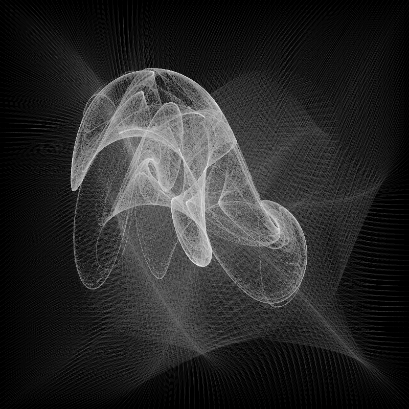
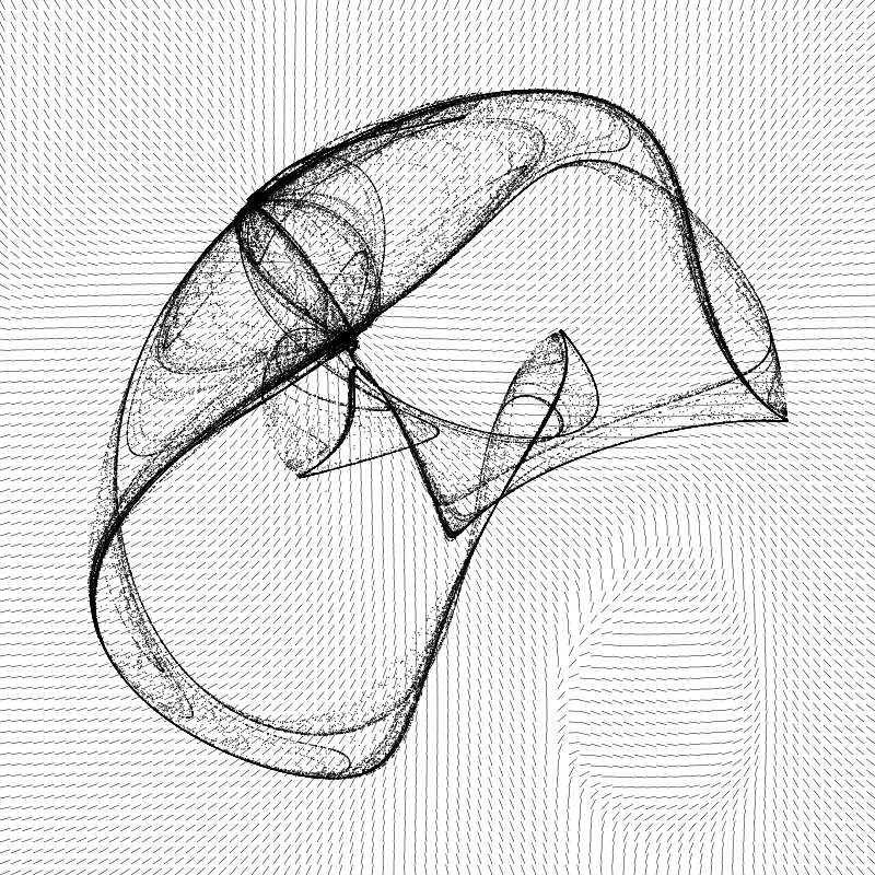
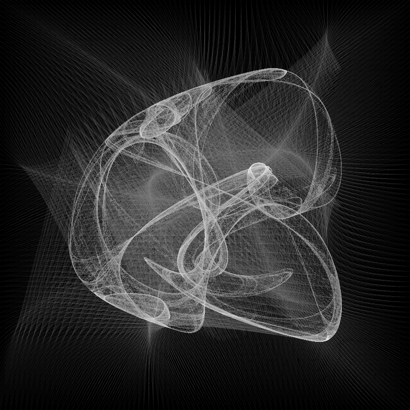
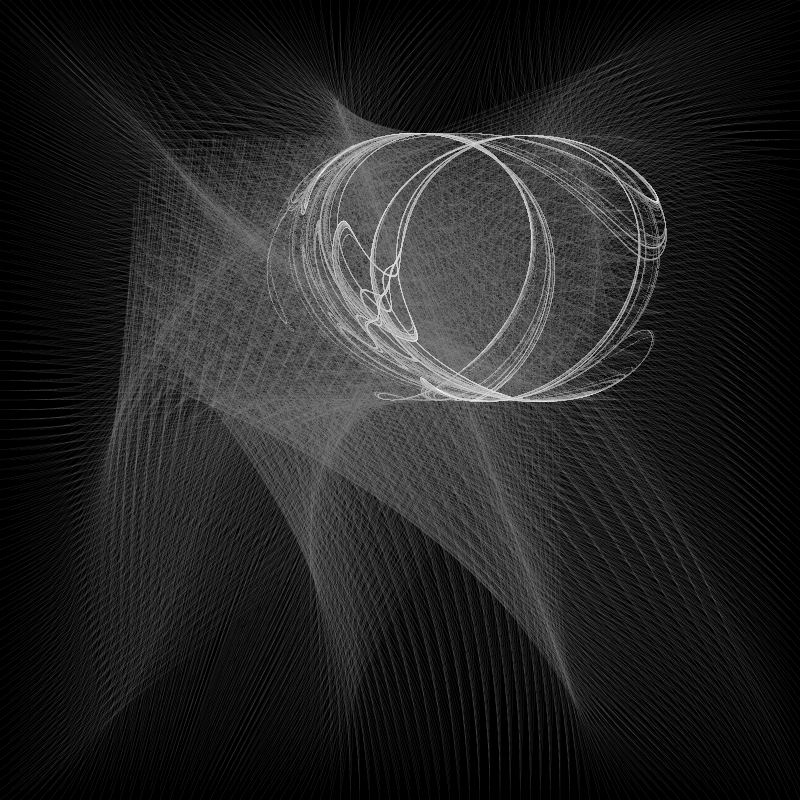
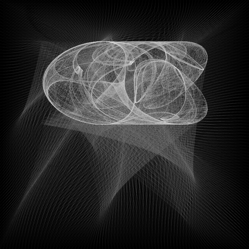
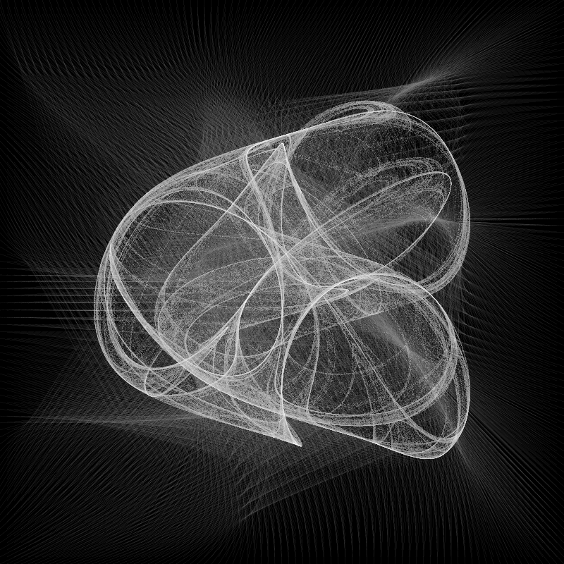
Finally, I decided to see what the field would look like if I rendered all the vectors at full length. I thought it would just be chaotic, but in fact, it’s quite beautiful.

These are rendered with very thin, nearly transparent lines, which allows multiple lines in the same vicinity to accumulate and become more visible.

To be honest, I was stunned when I first looked at this render. Not only was I surprised that it wasn’t just a mess of lines, and not only is it visually appealing, but it seems to show the forces that are shaping the attractor. Almost as if you could suddenly see the structure of space time warping in a gravitational field.

OK, I’m a little excited and maybe exaggerating a bit. But I think this is very cool, and dare I say, could be important?

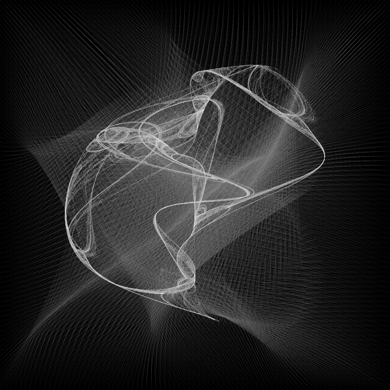
Here you can see the field and the attractor shape warping and twisting as one of the parameters is changed.

To end off, here’s a handful of images of the same attractor with random parameters, shown superimposed over their flow field. Click to view each one full size.

Summary

Being able to view these fields gives me so many new ideas to explore. Watch this space!