During my deep dive into Perlin and Curl noise, I kept bumping into the subject of Simplex noise. I figured it was worth going down that rabbit hole for a day or so. Here’s what I’ve found.

I guess it’s no surprise that Perlin noise was created by Ken Perlin. He came up with it in 1983. Later, in 2001, he went on to release Simplex noise. Although it was developed as an improvement over Perlin noise, and it has many advantages, it seems like Simplex has never really taken on to the same degree, and Perlin noise appears to maintain its place as the de facto standard.

Here are some of the advantages that were designed into Simplex noise:

• Simplex noise has a lower computational complexity and requires fewer multiplications.
• Simplex noise scales to higher dimensions (4D, 5D) with much less computational cost: the complexity is O(n²) in n dimensions instead of the O(n^{2^n}) of classic (Perlin) noise.
• Simplex noise has no noticeable directional artifacts (is visually isotropic), though noise generated for different dimensions are visually distinct (e.g. 2D noise has a different look than 2D slices of 3D noise, and it looks increasingly worse for higher dimensions).
• Simplex noise has a well-defined and continuous gradient (almost) everywhere that can be computed quite cheaply.
• Simplex noise is easy to implement in hardware.

– from: https://en.wikipedia.org/wiki/Simplex_noise

To explore these two, I created a little app that lets you compare and contrast the two in one and two dimensions. Actually, it uses 3d noise for each, but only displays one 2d slice at a time. I was not initially aware of the third bullet point above. Perhaps I’ll explore that difference in a future post.

Here’s the app:

Round 1 – 1D Noise

Initially the app is in 1d mode. Let’s take a screenshot so we know we’re looking at the same thing.

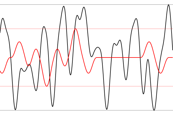
Here we have two plots of 1d noise. The black wavy line is Simplex noise. The red one is Perlin noise. There are a few important differences here.

1. The one that stands out for me is that plateau in the right hand side of the Perlin noise graph. It just hangs out at zero for a while. That’s not a rendering bug. Perlin noise just does that sometimes. Watch it long enough and you’ll see plenty of examples. Some way longer than that. As far as I can tell, Simplex just never does that. You might get a very brief leveling off, but it’s never that completely flat plateau like that. I’m pretty sure that’s one of the “dimensional artifacts” that Simplex was specifically designed to handle.
2. Next, you can see that Simplex noise just has a much larger range. You can see the peaks and valleys are way higher and lower than for Perlin noise. Those black horizontal lines running across the top and bottom of the image are the maximum and minimum values found for the Simplex noise thus far in the graph. Notice that they are nearly at the max and min range of the noise. Compare that to Perlin noise. The red horizontal lines show the range that it has extended to. It only covers about half the possible range.
3. Finally, Simplex noise is much more… active? You might say it has a higher wavelength, though that’s probably not the correct terminology. At any rate, for a given duration there are more peaks and valleys in Simplex than Perlin. In the above image, I count 13 peaks for Simplex and 8 (if I’m being kind) for Perlin.

Round 2 – 2D / 3D Noise

Now lets switch over to 2d noise. As I said above, this is really showing slices of 3d noise for each algorithm. Later I might do a test of 2d vs 3d for both. Again, let’s capture a screenshot and discuss.

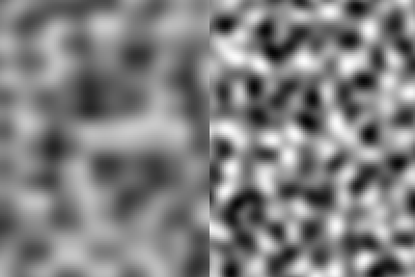
Perlin on the left, Simplex on the right.

Don’t mind the blockiness in some of the images. I kept the resolution low because I was animating it. It seems like the Simplex is more pixelated but that’s just because it has more contrast – more change happening in a smaller area – see below.

Immediately you can see all of the same issues we covered in 1d noise.

1. Right in the middle of the Perlin noise you can see a gray horizontal blob that extends through more than half of the image. That’s a dimensional artifact. Let’s change the scale and see if we can see more…

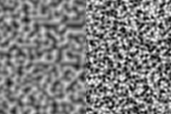
Here you can see several horizontal lines in the left hand Perlin sample. In both images, there are no blatant artifacts like this in the Simplex noise.

2. In both images you can see that the Simplex noise has more dark blacks, as well as more bright whites. The Perlin noise is pretty much just shades of mid-gray.
3. In both images, the Simplex noise is way busier. Again, wavelength, frequency, peak / valley count, whatever you want to call it, there’s more of it in Simplex.

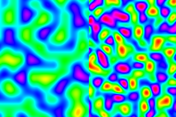
Finally, let’s revisit the image that you saw at the top of the post, it’s using color instead of grayscale.

Same things going on here. We seemed to avoid any serious artifacts this time, but you can see the different color ranges and complexity going on between the two.

Summary

Overall, I have to agree that Simplex has some great advantages. I’ve definitely been plagued by those artifacts in Perlin noise, and I like the increased range. The higher frequency or whatever isn’t really an advantage or disadvantage in my mind. You just need to scale your input a bit differently to get similar outputs. So you have to keep in mind that if you try to swap out Perlin for Simplex in an existing work, you might have to tweak it a bit to get the same look in terms of scale and dynamic range.

I’m also very curious about the “lower computational complexity”. Does this mean it’s more performant? I haven’t done any benchmarks, but that would be a big plus for sure.

I think you’ll be seeing a lot more Simplex noise round these here parts.

Source

Controls: MiniComps

Graphics: BLJS

Support this work