In my recent post on mapping Perlin noise to angles, I was put on to the subject of Curl noise, which I thought I understood, but did not. I figured out what Curl noise really was in a subsequent post and then posted my earlier incorrect (but still interesting and perhaps useful) concept of Curl noise in yet another post. Although I kind of understood what Curl noise was at that point, I wanted to give myself a more complete understanding, which I usually do by digging into the code, making sure I understand every line 100% and seeing what else I can do with it, trying to make multiple visualizations with it to test my understanding, etc.

I’ve read a lot on the subject of curl in the last week. Much of it was either super heavy with formulas and strange symbols, or really glossed over. In spite of having somewhat of a reputation as someone who is good at math (or maths for my UK brethren), I don’t have any formal background in the subject, so when someone starts throwing out the weird squiggly Greek letters that have some special meaning, or dives deep into mathematical jargon, I totally glaze over. I need to work out in my head what is happening, and kind of visualize it. Then I can write it down in layman’s terms – because those are the terms I understand. I found it best to work backwards from the code samples I found and comparing those to the formulas with all the Greek stuff. After a while, it started to make sense.

Finding the Slope on One Axis

We’ll start with general 2D Perlin noise. For any x, y location, you get a noise value from -1 to +1. Some libraries map that to a range of 0 to 1 instead, which is fine. I’m going to work with -1, +1. If you imagine that noise value as the height of the noise field at that location, you can then imagine a 3D landscape with mountains and valleys. And often enough, people use 2D Perlin noise for exactly that. So for any given x, y point, you’re on the slope of either some mountain or some valley. If you were actually there and looked around, in one direction you’d be looking uphill and in some other direction you’d be looking downhill. Theoretically, you might also be at the top of a mountain and everywhere you look is downhill, or at the bottom of a valley and all around you is up.

So let’s take one “slice” of this 2D landscape, as it moves across the x-axis. You could also consider this 1D Perlin noise, but let’s keep thinking of it as a slice of the 2D noise for now. It’s gonna look something like this:

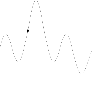
We’re at the x location indicated by the dot. You can see if we move to the right (increase x) we’ll be going “uphill”. And if we move to the left (decrease x) we’ll be going “downhill”. If we want to figure out what the slope is at that location, we could get a Perlin noise value for x minus a tiny amount (call that n1), and another noise value for x plus a tiny amount (call it n2). That would look like this:

We’ll call that “tiny amount” delta. So we have a small segment of noise going from x - delta to x + delta. The two noise value are n1 and n2. And you can see that n2 is higher than n1 in this case. So the slope of that noise segment is going up and to the right. It’s a positive slope.

In the following image, n2 is lower than n1, so we have a negative slope.

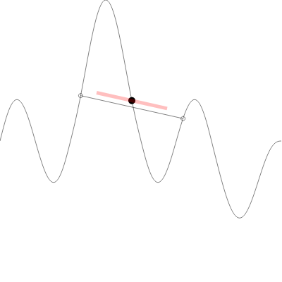
It’s important that the delta value be very small. If you start going out too far away in each direction, your slope will not be accurate. For example, in this image, there’s a red line that indicates the slope at the given point. You’d probably agree that it pretty closely matches the slope of the curve that that point.

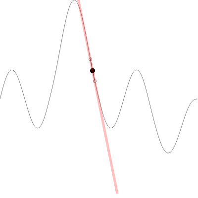
But here, in the next image, I’ve increased the delta significantly. The values for n1 and n2 are now so far away that they are on different slopes entirely. And the calculation for the slope at the main point is WAY off.

If you’re familiar with calculus, you’ve already recognized that what we’re trying to do here is find the derivative of the curve at that point. For many kinds of mathematical curves, you can figure out a formula that will give you the derivative at a given point. The curve itself is based on a formula and a lot of calculus has to do with finding the derivative formulas for given curve formulas.

I’m not sure if there is a way to do this for Perlin noise. But all the examples I have seen have done it using the above strategy, so I suspect this is the most straightforward method.

Disclaimer: I’ve studied some calculus, but I’m not standing on very solid ground here, so if I’ve said anything that’s way off, let me know and I’ll happily correct it.

If you want to play around with this concept and get a good feel for it, here’s the actual app that I used to make the above images:

To calculate the slope, you’d start with a given x value and delta value. From this you can get an x1 which is x - delta and x2 which is x + delta. Then you’d calculate n1 using Perlin noise for x1 and n2 using x2. Finally, the formula for the slop of a line, given two points is:

(y2 - y1) / (x2 - x1)

For us, this can be stated as:

(n2 - n1) / (delta * 2)

If the denominator doesn’t make sense to you, just remember that x2 is x+delta and x1 is x-delta. So x1 and x2 must be delta*2 apart from each other.

OK, now we have the slope … on the x-axis.

We can then do the same thing on the y-axis. I won’t belabor that point. It’s exactly the same thing.

But for the next step, we need to put the two vectors together.

Finding the Slope on Two Axes

The next example tries to visualize these slopes in 2D.

When this loads up it shows the Perlin noise field in the background and it will draw a red line starting at the mouse location. That line represents the slope at that point on the x-axis. I suggest you leave the settings as is at first and just see how it responds to the noise on the x-axis. Note that the line always runs “uphill” – or towards the whitest part of the noise field. Here’s a simplified version of the code that’s being used to draw that x-axis line:

const delta = 0.001;
const n1 = perlin(x - delta, y);
const n2 = perlin(x + delta, y);
const a = (n2 - n1) / (delta * 2);

context.beginPath();
context.moveTo(x, y);
context.lineTo(x + a * 40, y);
context.stroke();

The first part is exactly what I described in this article up to now. The variable a represents the slope on the x-axis.

The second part moves to the current mouse position (x, y), and draws a line to x + a * 40, y.

So if the slope, a is positive, the line will go to the right, and the higher it is, the longer the line. The value 40 there is arbitrary and just chosen to make sure the line is long enough to see clearly.

If the slope is negative, then the line will be drawn to the left, with the same rules for length. The result is that it is always drawn towards the higher part of the noise field than where the mouse currently is.

Note that if you move to the top of a hill (the lightest colored areas) or the bottom of a valley (the darkest areas), the line goes close to zero because the slope is leveling off before going in the opposite direction.

Once that seems to make sense, turn off “Show X” and turn on “Show Y” and see that it does the same thing on the y-axis. The simplified code for this is pretty similar.

const delta = 0.001;
const n1 = perlin(x, y - delta);
const n2 = perlin(x, y + delta);
const b = (n2 - n1) / (delta * 2);

context.beginPath();
context.moveTo(x, y);
context.lineTo(x, y + b * 40);
context.stroke();

Here, the variable b represents the slope on the y-axis, and we draw the line on the y-axis.

Finally, turn on “Show Slope”. This adds the x and y slope vectors together and draws a line that should go as steeply uphill as it can from the current location. It might help to turn off the x and y slopes and just see the resultant vector. Move the mouse around some more until you get a good feel on how it’s reacting to the noise field.

The code for this uses the exact same code for a and b as above, and the final slope line is drawn with:

context.beginPath();
context.moveTo(x, y);
context.lineTo(x + a * 40, y + b * 40);
context.stroke();

Onto the Curl! (finally)

Now we have a vector that points uphill from any given point. It’s what we’ve been calling (a, b) Finding the Curl noise vector is simple, just go 90 degrees – perpendicular – to that slope vector. You don’t even have to use any trig or anything here. For any vector (a, b), the perpendicular vector would be (b, -a).

If that doesn’t make sense to you, just draw it out a few times on a piece of graph paper. Draw a (2, 7) vector – a line that goes two units to the right and 7 units up (Cartesian coords, not screen coords). Then draw a (7, -2) vector. One that goes 7 units to the right and two down. If you did it right, they should form a right angle.

Yes, you could also do (-b, a). It will just go perpendicular in the other direction. Choose one. It’s up to you.

To see this action, go to the same demo above and click on the “Curl” radio button.

This will draw the slope vector in red and the curl vector in green. Here’s the code for drawing the curl vector.

context.beginPath();
context.moveTo(x, y);
context.lineTo(x + b * 40, y - a * 40);
context.stroke();

The path of a curl vector is kind of like one of those roads that’s cut into the side of the mountain. You’re driving along at a level grade. On one side you see the mountain towering above you, on the other side, the valley drops off below you. You’re moving perpendicular to the slope.

OK, so we are there, let’s see it all in action…

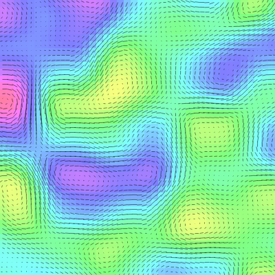
This is really the same basic functionality, but rather than plotting the slope of a single mouse location, we’re doing it for a grid extending across the whole field. And we’re animating the noise by moving through the z-axis. And using prettier colors.

In this case, the yellowish areas are the valleys and the reddish purple areas are the peaks. In slope mode, the lines are always pointing uphill to the purple, away from the yellow.

Play with the settings till you get a feel for it, and then switch over to curl mode. Now you see lines circling the peaks and valleys, just like those mountain roads. These are sometimes called vortexes (or vortices).

This explains the non-compression aspect of Curl noise that I talked about in an earlier post. It’s like having multiple parallel mountain roads. When you’re at a given level on the slope, you’ll tend to stay on that level. If someone is traveling along beside you, they’ll be on another road a bit higher or lower on the mountain than you are, and you’ll generally stay separate.

Also, try cranking up the line width and turning the resolution all the way down, then pushing up the noise speed. It has nothing much to do with this tutorial, but it looks pretty cool.

The Code

The code I shared in this post is just a few excerpts and very much simplified for clarity. The full code for all the examples is here: https://github.com/bit101/curlnoise_tutorial. It’s kind of hacked together, optimized for… well optimized for my brain. Not nearly production ready, but hopefully lucid enough for you to glean some knowledge from.

Controls: MiniComps

Graphics: BLJS

Support this work